An index value needs an uncertainty model
An NDVI value can be calculated to many decimal places from two reflectance estimates. Those decimals describe numerical precision, not confidence in the observation. To decide whether a small difference between two index values is informative, an analyst also needs to understand the uncertainty of the inputs and how their errors relate. Red and near-infrared measurements are not necessarily affected independently, particularly when processing or calibration influences both channels.
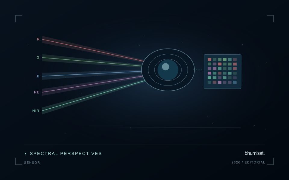
This tutorial develops a two-input uncertainty calculation with invented reflectance values. It is a teaching example, not a calibration result for any satellite. For BhumiSat's research and concept-design programme, the calculation illustrates questions that a future multispectral processing chain would need to answer. BhumiSat is studying a 3U CubeSat concept with RGB, Red Edge and NIR sensing and a mission vision for 2030. Its final sensor specifications, calibration performance and operational data products are not confirmed.
Define the reflectance inputs and the intended result
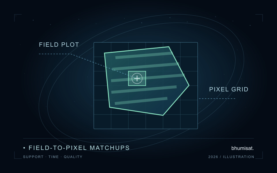
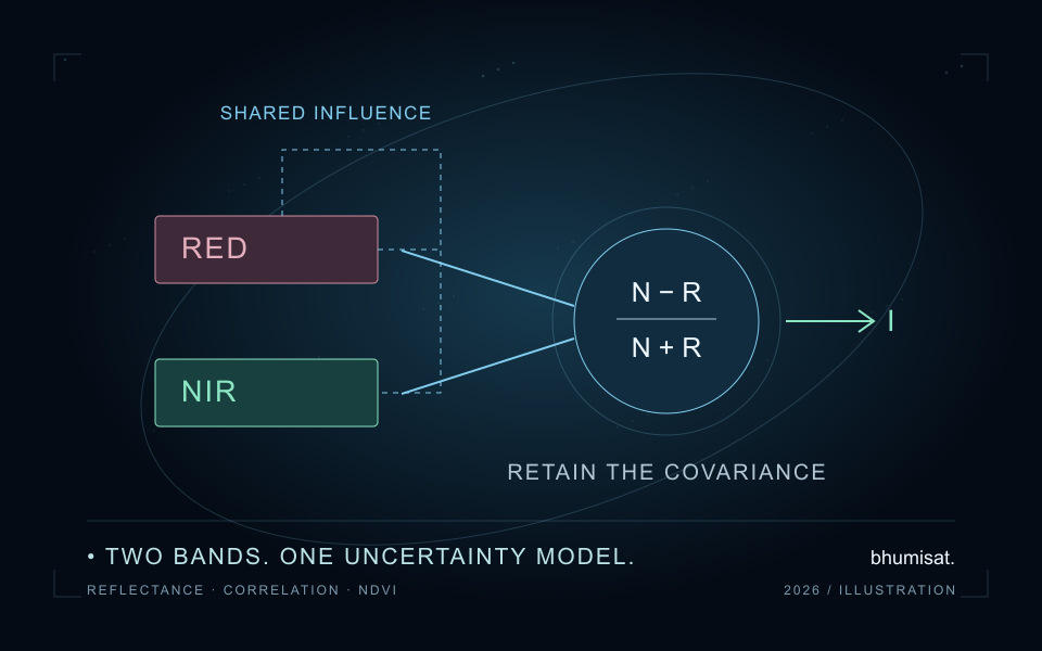
USGS defines NDVI as near-infrared minus red divided by near-infrared plus red. Here N denotes the near-infrared reflectance estimate, R denotes red reflectance and I denotes the resulting index: I = (N − R)/(N + R). The example uses dimensionless reflectance fractions rather than scaled integers. The two channels must describe a compatible observation and spatial support; inserting numbers from different dates or misaligned grids would create a different measurement problem. [1]
Record the product level, bands, scaling and any offsets applied before the ratio. An uncertainty supplied for encoded digital values cannot simply be attached to physical reflectance without converting its units and considering the conversion model. Likewise, uncertainties in atmospheric correction, calibration and registration describe different influences. Name which are represented by the proposed input uncertainties and which remain outside the calculation. A short model with clearly stated limits is easier to assess than a complete-looking number with an unclear meaning.
Retain covariance in the propagation equation
NIST's law of propagation of uncertainty combines input standard uncertainties through sensitivity coefficients and includes covariance between inputs. It is based on a first-order approximation of the measurement equation. For two NDVI inputs, define a as the derivative with respect to N and b as the derivative with respect to R. The combined variance is a squared times the variance of N, plus b squared times the variance of R, plus twice a times b times their covariance. [2]
Differentiating the ratio gives a = 2R/(N + R)² and b = −2N/(N + R)². If the input standard uncertainties are u(N) and u(R), write their covariance as rho times u(N) times u(R). Rho is a correlation coefficient between the input errors represented by this model. It is not the correlation between red and NIR values across a landscape, where real differences in vegetation and soil can drive the relationship.
Calculate three scenarios with the same band uncertainties
Set N to 0.50 and R to 0.20, giving an NDVI of approximately 0.4286. Assign each input a standard uncertainty of 0.01 in reflectance units. The sensitivity coefficients are approximately 0.8163 for N and −2.0408 for R. Because their signs differ, positive covariance contributes a negative cross term to this particular output variance. That does not make covariance optional: its sign and magnitude are part of the model.
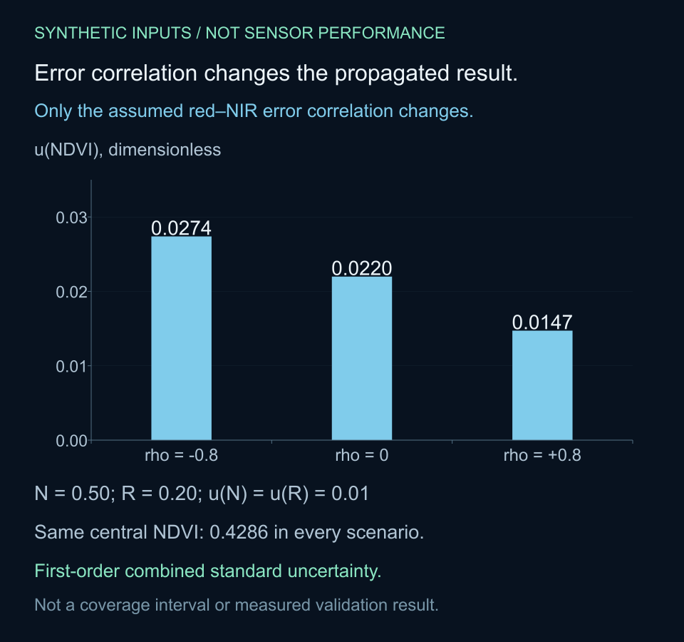
Using rho values of −0.8, zero and +0.8 gives approximate combined standard uncertainties of 0.0274, 0.0220 and 0.0147 respectively. All three scenarios have the same central reflectance estimates and individual standard uncertainties. The difference comes entirely from the assumed error relationship. These are calculated alternatives for an invented case; none is a measured correlation or an accuracy specification. Selecting the smallest result because it looks preferable would be choosing an assumption to obtain a desired answer.
Distinguish a shared gain from a shared offset
A common multiplicative factor provides a useful algebra check. Multiplying both N and R by the same nonzero gain leaves this ratio unchanged, because the factor cancels between numerator and denominator. A gain of 1.05 therefore leaves the example's NDVI at approximately 0.4286. This cancellation applies to that precisely defined common influence. It does not imply that NDVI is insensitive to channel-dependent gains, imperfect corrections, geometry or all other measurement effects.
A common additive offset behaves differently. Adding 0.01 to both channels preserves the numerator but increases the denominator, producing an index of approximately 0.4167 in the example. The same phrase, shared calibration error, can therefore describe influences with different consequences. The JCGM Guide discusses correlations arising from common instruments or reference quantities and the option of including shared influences explicitly in the measurement model. Identify the physical influence rather than assigning correlation solely from its name. [3]
Check where the local approximation is defensible
The derivatives are evaluated at the estimated reflectances, so the result describes local sensitivity. Near a small red-plus-NIR denominator, the ratio can respond strongly and nonlinearly to input changes. A first-order calculation can then be an inadequate description of the output distribution. The JCGM Guide explicitly notes that significant nonlinearity requires consideration beyond a first-order treatment. Examine the function over the range supported by the input model before presenting the result as a dependable summary. [3]
A distribution-based evaluation would require justified joint input distributions, including their dependence, and a policy for physically or procedurally invalid samples. This article does not claim to perform that evaluation. Its short Python calculation deliberately accepts only finite nonnegative reflectances with a positive sum and finite nonnegative standard uncertainties. Those guards define the toy example's domain; they are not a universal rule for every reflectance product or a substitute for reading its quality flags.
Run the calculation and preserve the assumptions
The accompanying Python example uses only the standard library. It evaluates the analytic derivatives, retains the covariance term and prints the three correlation scenarios. It also recalculates the ratio after the shared gain and offset transformations. All values are invented, and the chart displays the same first-order standard uncertainties. It does not show measured error bars, a coverage interval or performance demonstrated by BhumiSat or another instrument.
Keep the input values, uncertainty units, rho assumption, formula version and output together when adapting this calculation. Check a simple case by hand and verify numerical derivatives against small perturbations of the ratio. If a model produces a negative variance beyond rounding effects, inspect the covariance structure and implementation rather than hiding it with an unconditional absolute value. With more than two inputs, a collection of individually plausible pairwise correlations also needs to form a valid joint covariance model.
# Invented positive-reflectance example; first-order propagation only.
from math import isfinite, sqrt

def ndvi(nir, red):
    return (nir - red) / (nir + red)

def standard_uncertainty(nir, red, u_nir, u_red, rho):
    values = (nir, red, u_nir, u_red, rho)
    if not all(isfinite(v) for v in values):
        raise ValueError("Inputs must be finite")
    if min(nir, red, u_nir, u_red) < 0 or nir + red <= 0:
        raise ValueError("Outside this example's input domain")
    if not -1 <= rho <= 1:
        raise ValueError("Correlation must lie between -1 and 1")
    a = 2 * red / (nir + red) ** 2
    b = -2 * nir / (nir + red) ** 2
    variance = (a * u_nir) ** 2 + (b * u_red) ** 2
    variance += 2 * a * b * rho * u_nir * u_red
    return sqrt(max(0.0, variance))  # valid 2-input model; guard roundoff

nir, red = 0.50, 0.20
print(f"NDVI={ndvi(nir, red):.4f}")
for rho in [-0.8, 0.0, 0.8]:
    u = standard_uncertainty(nir, red, 0.01, 0.01, rho)
    print(f"rho={rho:+.1f}: u(NDVI)={u:.4f}")
print(f"Shared gain: {ndvi(1.05 * nir, 1.05 * red):.4f}")
print(f"Shared offset: {ndvi(nir + 0.01, red + 0.01):.4f}")
# NDVI=0.4286
# rho=-0.8: u(NDVI)=0.0274
# rho=+0.0: u(NDVI)=0.0220
# rho=+0.8: u(NDVI)=0.0147
# Shared gain: 0.4286
# Shared offset: 0.4167
Do not turn standard uncertainty into an automatic change claim
NIST distinguishes combined standard uncertainty from a coverage statement: interpreting an interval around a result requires assumptions about its distribution and the reliability of the uncertainty estimate. A standard uncertainty is therefore not automatically a 95 percent interval. Report what the number represents and how it was obtained. If an expanded uncertainty is reported, state the coverage factor and the basis for the associated coverage interpretation rather than silently relabelling a standard deviation. [4]
A comparison between dates introduces another dependence question. The uncertainty of an index difference depends on the two index uncertainties and their cross-date covariance. A persistent shared calibration influence may affect those dates together, while cloud contamination or registration can behave differently. Field averaging likewise requires attention to spatial dependence; adding pixels does not automatically remove a common influence. Keep those additional models separate from the two-band example instead of treating its output as a complete uncertainty budget for change detection.
Use the budget to guide calibration research
For an early multispectral mission study, the useful outcome is an evidence plan. List the candidate influences on each band, identify shared references or processing steps and design measurements that can characterise their effects. Where feasible, estimate uncertainty components and covariance from appropriate calibration evidence rather than from spatial correlation in an arbitrary image. Keep results traceable to the instrument configuration and processing version under which they were obtained.
For BhumiSat, that work belongs alongside application validation and payload concept development. A vegetation-index tutorial can expose which calibration information a user would need, but it cannot establish a future spacecraft's accuracy. The defensible conclusion is conditional: NDVI uncertainty depends on the chosen input model, and retaining red–NIR error covariance can materially change the result. Preserve that model with the index so its numerical precision can be distinguished from the evidence supporting its interpretation.
Sources & further reading
Review multispectral sensing concepts, connect the index to field-to-pixel validation, or explore BhumiSat's research questions for its 2030 vision.