Start with a comparison you can explain
A field visit and a satellite acquisition do not automatically describe the same crop condition. An observer may measure several plants beside an access track, while a satellite pixel includes canopy, exposed soil and part of a neighbouring parcel. Both records can be correct within their own measurement domains. The difficulty begins when a spreadsheet places them beside each other and quietly treats them as equivalent. A useful Sentinel-2 field validation workflow makes those domains explicit before calculating an error statistic.
This tutorial develops a practical design for a crop matchup table: one auditable record connecting a field observation, a selected satellite acquisition and a documented area of comparison. The workflow and numerical example below are proposed teaching methods, not results from a field campaign. They are relevant to BhumiSat's application research, but they do not demonstrate BhumiSat sensor performance. BhumiSat remains a TechnoGIS Earth observation initiative studying a CubeSat concept and a mission vision for 2030.
Define the variable before choosing the pixel
Write the intended comparison as a sentence. For example: compare independently measured canopy leaf area index with an estimated leaf area index over a specified plot, for a specified acquisition. This is different from comparing leaf area index directly with NDVI. NDVI is a spectral index; leaf area index describes canopy structure. A fitted relationship may connect them, but its output, assumptions and training domain must be stated. A strong correlation between unlike quantities does not establish that either quantity has been retrieved without bias.
The CEOS Land Product Validation subgroup describes reference measurements and upscaled reference maps as distinct resources. Its biophysical validation page also identifies uncertainty and independence as central to fiducial reference measurements. Use that distinction to design the table: retain the original instrument readings separately from the plot reference estimate and record how the latter was produced. A reference estimate should have its own quality assessment rather than being treated as an exact answer merely because someone collected it on the ground. [4]
Freeze the product identity and reflectance convention
Select a specific Sentinel-2 Level-2A product and retain its complete identifier, sensing time, tile and processing baseline. Copernicus describes Level-2A as atmospherically corrected surface reflectance with supporting quality information. The product documentation also gives the conversion from encoded digital numbers using the band offset and quantification value recorded in metadata. Preserve those inputs when working from downloaded products. Do not infer a universal conversion solely from the appearance of an image or a filename date. [1]
Hosted collections can apply their own documented transformations. Google's COPERNICUS/S2_SR_HARMONIZED documentation states that newer scenes are shifted into the range of older scenes and lists reflectance bands with a scale factor of 0.0001. Record that collection identity if you use it; applying an original-product offset again would mix conventions. For a basic NDVI exercise, identify the red and near-infrared bands explicitly. In this collection B4 and B8 are listed at 10 metres, while red-edge B5 is listed at 20 metres. [3]
Make spatial support a saved object
Store the field boundary and the actual sampled plot as separate geometries. A whole farm boundary is an administrative object; it is not evidence that a few readings represent the whole farm. Record the coordinate reference system, survey method, instrument footprint and sampling layout. If several plots represent different parts of a field, retain those identities through aggregation. An area estimate, boundary version and positional uncertainty note make later interpretation much easier when a parcel is edited or surveyed again.
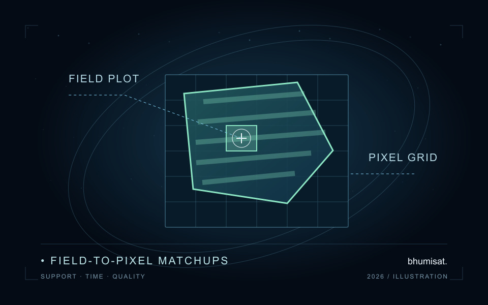
Overlay the plot with the selected raster grid in a suitable projected coordinate system. Decide whether the comparison uses complete interior cells or fractional overlaps with the plot, then save that rule and the participating cell identifiers. A drawn pixel square is a useful accounting unit, but the real instrument response and geolocation are more complex than a perfectly bounded box. Inspect field edges and repeat the extraction under plausible positional shifts. Treat the change as a sensitivity result, not as a reason to choose whichever alignment improves agreement.
Combining bands also requires a declared analysis grid. Upsampling a 20-metre band onto a 10-metre grid changes the storage grid without creating independent 10-metre observations. Preserve the source resolution and resampling method in the table. If you analyse NDVI at its chosen grid and a red-edge index at a different grid, keep separate support identifiers. Sharing a field name is insufficient to prove that two index summaries describe the same area.
Match time with an agronomic reason
Keep the field measurement timestamp and satellite sensing timestamp, including time zones, rather than joining only on a calendar date. Also record the interval during which a field campaign was collected. A morning measurement and an afternoon measurement may differ in illumination or canopy condition; observations separated by several days can cross irrigation, harvest or a rapid growth stage. The acceptable difference therefore follows the variable and crop process being studied, not a convenient fixed number of days copied from another project.
Set the temporal acceptance rule before looking at model residuals. Record a reason for each accepted exception, such as a documented stable canopy period, and retain rejected candidate acquisitions with a rejection code. If a cloud-free acquisition falls outside the defensible window, report that no valid matchup exists. Filling the gap with a distant clear image can create an apparently complete dataset while changing the scientific question. Missingness is a result that should remain visible in the study's accounting.
Screen quality locally and retain the denominator
A scene-wide cloud percentage is useful for finding candidates, but the field itself needs a local quality check. Copernicus documents the Level-2A Scene Classification Layer at 20 metres, with labels including cloud shadow, vegetation, non-vegetated surfaces, water, cloud classes and snow or ice. Save the actual classes encountered and your acceptance rule. Class labels are processing outputs, so they should support visual inspection and method documentation rather than silently becoming infallible ground truth. [2]
Define the mask for the intended comparison. A vegetation-only rule could remove bare gaps that legitimately belong to the sampled field and inflate a field average. Conversely, retaining a shadowed or cloudy part can distort the spectral summary. Use categorical resampling when transferring class labels onto another grid, record that method, and inspect mask boundaries. If a conservative cloud-neighbour exclusion is added, record its distance and rationale. No single mask setting is a universal guarantee of clean crop observations.
For every extraction, retain both the candidate overlap area and the area remaining after screening. Their ratio is the valid-area fraction. Also save the accepted and rejected cell counts, but remember that fractional edge cells contribute different areas. A mean calculated from the clear corner of a field should be described as a mean over that retained support. Comparing it with a full-field reference requires a separate justification; a high valid-area fraction alone does not prove representativeness.
Check one small aggregation by hand
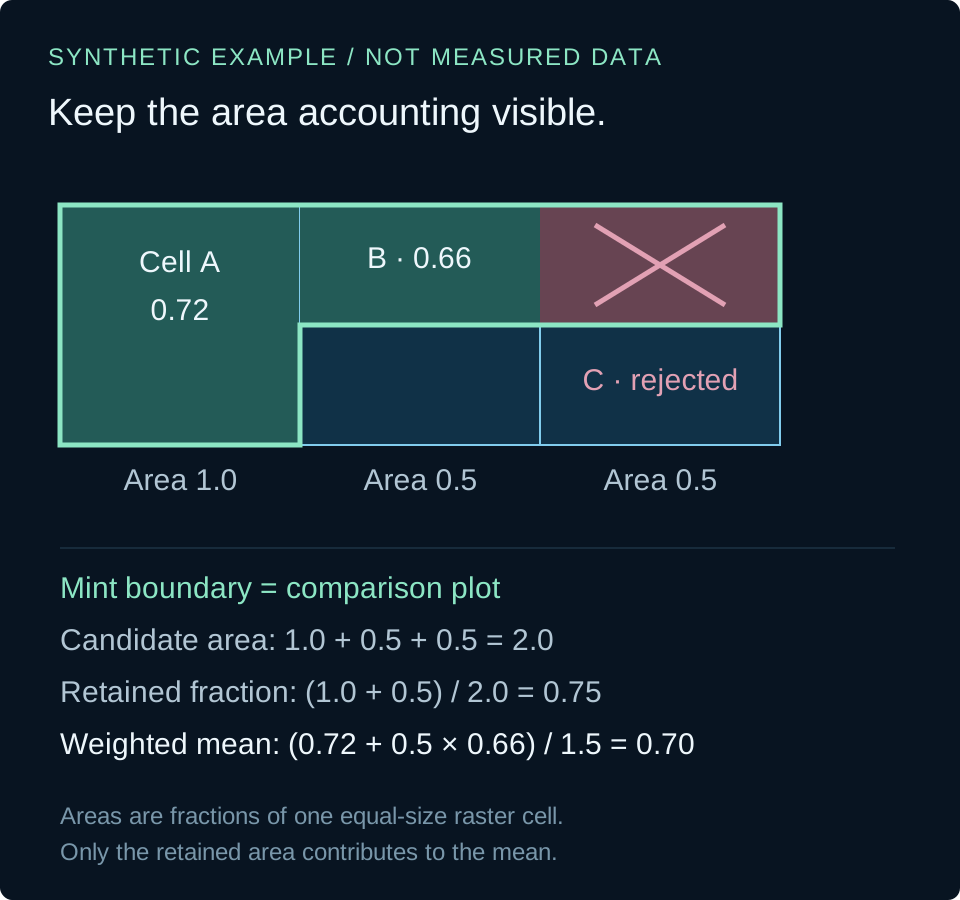
Consider a synthetic plot overlapping three equal-size raster cells. The overlap areas, expressed in units of one full cell area, are 1.0, 0.5 and 0.5. Their illustrative index values are 0.72, 0.66 and 0.20. Suppose the third cell fails the declared quality rule. Candidate area is 2.0 units and retained area is 1.5 units, giving a valid-area fraction of 0.75. The overlap-weighted retained mean is 0.70. The simple unweighted mean of the two accepted values would instead be 0.69.
This small difference is useful because it makes the accounting testable. The rejected value must contribute neither to the retained numerator nor to its denominator. An extraction with no retained area should return a missing result and an explicit rejection reason, never a zero that could be mistaken for a physical index. The short Python example implements only this arithmetic using invented inputs. It does not download imagery, select cloud classes, perform geospatial intersections or estimate an agronomic variable.
The example averages per-cell index values. Calculating an index from area-averaged red and near-infrared reflectance is a different operation and can give a different answer because the index is a ratio. Name the aggregation order in the matchup record. Before processing hundreds of fields, inspect a few cells manually, including one edge overlap and one masked cell. That exercise often reveals a denominator or support error that a smooth-looking map would conceal.
# Synthetic arithmetic only; areas use one full cell as the unit.
cells = [(1.0, 0.72, True), (0.5, 0.66, True), (0.5, 0.20, False)]
candidate_area = sum(area for area, value, valid in cells)
retained_area = sum(area for area, value, valid in cells if valid)
mean = (sum(area * value for area, value, valid in cells if valid)
        / retained_area) if retained_area else None
fraction = retained_area / candidate_area if candidate_area else None
print(f"mean={mean:.2f}, valid_fraction={fraction:.2f}")
# mean=0.70, valid_fraction=0.75
Save a table that supports an honest error analysis
Give every row a stable matchup identifier. At minimum retain the field and plot identifiers, boundary version, reference variable and units, reference value and uncertainty description, reference timestamp, satellite product identifier, sensing timestamp, processing convention, grid definition, support identifier, quality rule, candidate area, retained area, summary value and decision reason. Keep the extraction settings and software version alongside the table so another analyst can reconstruct a row without depending on a screenshot or an undocumented desktop session.
Keep model fitting separate from final evaluation. If an empirical relationship was trained with a field's observations, do not present those same observations as independent validation. Repeated visits to one field also share context, so treating every row as an unrelated replicate can exaggerate the amount of evidence. Design a held-out evaluation around the intended transfer question, such as a new field or season, and report the number of distinct fields and dates as well as the number of rows.
When satellite estimates and references represent the same variable, units and support, inspect signed differences and absolute differences before reducing them to a single score. Plot residuals against time separation, retained fraction and field-edge sensitivity. State whether reference uncertainty is quantified or only described qualitatively, and distinguish model disagreement from a complete uncertainty budget. Report rejected matchups by cause. A study that explains its exclusions and limits is easier to improve than one that reports only a favourable correlation.
Use the workflow to ask better mission questions
For BhumiSat's research, the immediate value of this exercise is a clearer set of observation requirements. If most failures arise from mixed parcel edges, application studies can investigate spatial support. If rapid crop changes dominate the mismatch, observation timing becomes a question to study. If usable coverage collapses under quality screening, the delivery requirement should include the frequency of valid observations. These findings can guide concept discussions without claiming that a proposed payload has already met those requirements.
Keep the distinction between existing Sentinel-2 evidence and a future BhumiSat mission explicit. Performance demonstrated with one sensor, processing chain and field campaign does not automatically transfer to another spacecraft. A traceable matchup table provides a reusable way to investigate that gap: define the variable, preserve geometry and time, screen locally, account for retained area and evaluate independently. That sequence turns a field visit and an image into a comparison whose meaning can be checked, challenged and improved.
Sources & further reading
Continue with crop monitoring and field validation, explore satellite, drone and field data integration, or read about the questions behind BhumiSat's 2030 vision.