Separate the map count from the area estimate
A forest-loss map can look convincing and achieve a high overall accuracy while still missing a substantial share of the loss relevant to a study. Counting its labelled pixels answers how much area the map assigns to loss. Estimating how much loss occurred requires reference evidence and an analysis that respects how that evidence was sampled. The difference matters when a relatively uncommon change is surrounded by a much larger area labelled as unchanged.
This tutorial uses an invented two-class example to make that distinction numerical. It does not analyse a real forest or establish any country's loss rate. Its relevance to BhumiSat is methodological: application research should define how delivered imagery would support an independently evaluated land-change result. BhumiSat remains a TechnoGIS research and concept-design initiative studying a multispectral 3U CubeSat and a mission vision for 2030, without confirmed operational imagery or final spacecraft specifications.
Define the frame and the reference label first
Specify the reporting boundary, observation interval, assessment unit and meaning of loss before collecting validation labels. A canopy disturbance label is not automatically a conclusion about permanent land-use conversion or its cause. In this example, assume a fixed, correctly defined eligible frame of ten thousand hectares, partitioned into equal-area units. Every unit receives a binary loss or not-loss label for one declared interval. Errors in defining the eligible frame are outside this deliberately limited example.
Reference labels need appropriate evidence for both ends of that interval and for the spatial unit being assessed. Record ambiguous cases rather than resolving them solely by agreeing with the map. FAO's Remote Sensing Survey methodology describes interpretation by trained national experts and quality control with external reinterpretation. That illustrates why a reference process deserves its own quality checks. An alternative image is not automatically a flawless reference, particularly if it shares the original map's timing or visibility limitations. [4]
Keep the probability design with the samples
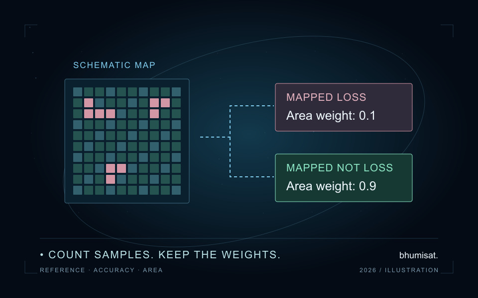
Assume the map labels one thousand hectares as loss and nine thousand as not loss. Use those mapped classes as two non-overlapping sampling strata with known area weights of 0.1 and 0.9. Imagine selecting fifty equal-area assessment units by simple random sampling within each stratum, independently between strata. The equal allocation deliberately represents the smaller stratum more intensively. It does not make the two strata equal in landscape area.
Save the frame, stratum areas, inclusion rules, selection procedure and sample identifiers before interpretation. SEPAL's sampling documentation explicitly separates designing sample locations from collecting reference observations and calculating final estimates. It also defines stratum weights from mapped area. Keep that distinction in a local workflow: exporting a point layer does not finish validation, and a convenient set of roadside visits cannot simply inherit the statistical interpretation of a probability sample. [2]
Convert the invented counts into area proportions
In the fifty samples from mapped loss, suppose the reference labels forty as loss and ten as not loss. In the fifty from mapped not loss, suppose five are reference loss and forty-five are reference not loss. With rows defined as mapped strata and columns as reference classes, the count matrix is therefore forty, ten in its first row and five, forty-five in its second. These are invented labels, not observations collected for this article.
For this design, multiply each row's reference proportions by that row's area weight. The estimated landscape proportions become 0.08 and 0.02 in the mapped-loss row, and 0.09 and 0.81 in the mapped-not-loss row. They sum to one and their row totals recover 0.1 and 0.9. Olofsson and colleagues describe this area-proportion approach for stratified accuracy assessment. Writing both axis definitions beside the matrix is essential because software interfaces do not all use the same orientation. [1]
Read omission and commission alongside overall accuracy
The estimated correct landscape proportion is the sum of the diagonal, 0.08 plus 0.81, giving 89 percent overall accuracy. Simply pooling the hundred sample records gives eighty-five agreements and an 85 percent score. That pooled fraction does not estimate landscape accuracy under this unequal-intensity allocation. The smaller mapped-loss stratum contributes half the sample but only one tenth of the area, so its records cannot have the same landscape weight as records from the other stratum.
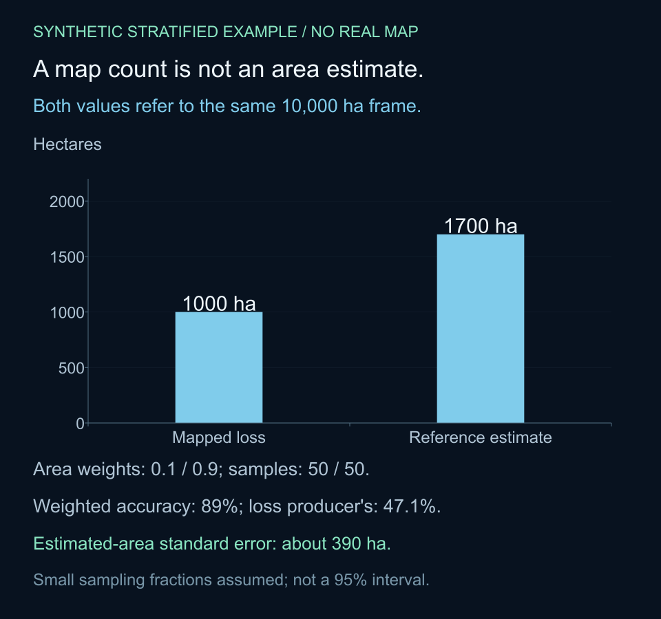
For mapped loss, estimated user's accuracy is 0.08 divided by its mapped proportion of 0.10, or 80 percent. Estimated producer's accuracy for reference loss is 0.08 divided by the reference-loss column total of 0.17, or about 47.1 percent. The high overall score therefore coexists with substantial estimated omission of loss. These metrics answer different questions; reporting only the most favourable one would conceal an important limitation of the example map.
Estimate loss area without relabelling every pixel
Adding the reference-loss column gives an estimated loss proportion of 0.17. Multiplying by the ten-thousand-hectare frame yields an estimated 1,700 hectares, compared with the map's direct count of 1,000 hectares. The arithmetic explains the difference: an estimated 200 hectares labelled as loss are reference not loss, while an estimated 900 hectares of reference loss lie in the much larger mapped-not-loss stratum. Subtracting the former and adding the latter gives the same estimate.
This is a statistical area estimate conditional on the assumed design and reference process. It does not identify which unsampled pixels are wrong, nor does it supply a corrected spatial map. Keep the original map and the area estimate as separate outputs. SEPAL's analysis documentation likewise distinguishes map pixel counts from stratified estimates and reports accuracy and area information together. An area result should retain its sample basis rather than appearing to be a newly verified label for every location. [3]
Calculate sampling precision under the stated design
The estimated area varies across possible samples. For the simple stratified design used here, an approximate variance of the loss proportion sums each squared area weight multiplied by the within-stratum loss proportion times one minus that proportion, divided by the stratum sample size minus one. This calculation omits finite-population corrections, assuming the sampling fractions are small. It gives an area standard error of approximately 390 hectares for the invented counts. It is not a complete uncertainty assessment of a real forest-loss study. [1]
The Python example retains those assumptions and prints the weighted matrix, accuracy measures, area and approximate standard error. No imagery is downloaded and no random sample is actually drawn. Fifty samples per stratum is a teaching choice rather than a recommendation for every project. Sampling precision depends on allocation and observed class occurrence, while reference-label error and frame exclusions require additional assessment. A standard error alone should not be presented as a 95 percent interval without an appropriate interval method and its assumptions.
# Invented equal-area units; independent simple random samples in each stratum.
# Rows: mapped loss / mapped not loss. Columns: reference loss / not loss.
from math import sqrt

area_ha = 10_000
weights = [0.1, 0.9]
counts = [[40, 10], [5, 45]]
sizes = [sum(row) for row in counts]
assert abs(sum(weights) - 1) < 1e-12 and all(n > 1 for n in sizes)
proportions = [[weights[i] * value / sizes[i] for value in row]
               for i, row in enumerate(counts)]
loss_fraction = sum(row[0] for row in proportions)
overall = sum(proportions[i][i] for i in range(2))
pooled = sum(counts[i][i] for i in range(2)) / sum(sizes)
user_loss = proportions[0][0] / weights[0]
producer_loss = proportions[0][0] / loss_fraction
within_loss = [counts[i][0] / sizes[i] for i in range(2)]
variance = sum(weights[i] ** 2 * p * (1 - p) / (sizes[i] - 1)
               for i, p in enumerate(within_loss))  # omit finite-population correction
print("Area-proportion matrix:", [[round(v, 2) for v in row] for row in proportions])
print(f"Pooled agreement={pooled:.1%}; weighted accuracy={overall:.1%}")
print(f"Loss user's accuracy={user_loss:.1%}; producer's={producer_loss:.1%}")
print(f"Mapped loss={area_ha * weights[0]:.0f} ha")
print(f"Estimated loss={area_ha * loss_fraction:.0f} ha")
print(f"Approximate area standard error={area_ha * sqrt(variance):.1f} ha")
# Area-proportion matrix: [[0.08, 0.02], [0.09, 0.81]]
# Pooled agreement=85.0%; weighted accuracy=89.0%
# Loss user's accuracy=80.0%; producer's=47.1%
# Mapped loss=1000 ha
# Estimated loss=1700 ha
# Approximate area standard error=389.9 ha
Preserve the design when handling difficult observations
Do not silently drop cloud-obscured reference sites or replace them with nearby convenient locations. Record unresolved units and use a response procedure compatible with the sampling design. Likewise, labels used to tune the classifier should not quietly reappear as an independent test of its final accuracy. Freeze the evaluated map version and retain the interpretation evidence so a later review can distinguish model improvement from a change in the validation process.
For a reproducible handoff, save the reporting boundary and area method, class definitions and dates, sampling frame and allocation, selection information, reference labels, quality decisions and matrix orientation. Retain both sample-count and estimated-area matrices with clear units, plus the estimator and precision calculation. If the actual design uses clusters, unequal selection probabilities, polygons or mixed labels, this simple equal-area-unit code is not a general replacement for an estimator matched to that design.
Turn map validation into application requirements
For BhumiSat's land-monitoring research, the example suggests an evidence plan rather than a spacecraft performance claim. Decide which changes matter, what independent reference information is available and how area uncertainty will be reported. A useful application can require more than visually clear imagery: consistent timing, traceable processing, suitable spatial support and a defensible reference sample all influence what the final result can mean.
The practical lesson is to keep three statements distinct: how much loss the map labels, how accurately it identifies the target class and what area the reference sample estimates under its design. In this invented case, 89 percent overall accuracy does not make a 1,000-hectare map count equivalent to the 1,700-hectare stratified estimate. Reporting the weights, class errors and sampling precision makes that difference visible and gives the next research step a concrete purpose.
Sources & further reading
Connect map assessment to traceable field-to-pixel validation, explore the assumptions behind an index uncertainty model, or read BhumiSat's research questions for its 2030 vision.