Budget the journey from exposure to usable data
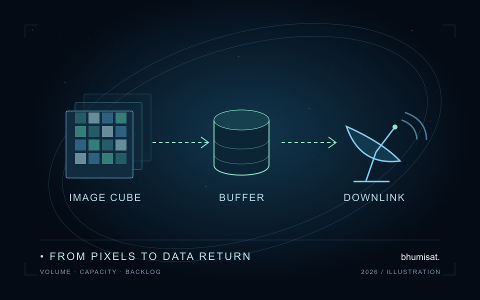
A multispectral image has to travel through more than an optical system. Samples leave a detector, enter memory, wait for communication opportunities and eventually become files that a ground processor can verify. An impressive radio data rate does not by itself show how many complete observations a mission could deliver. A CubeSat image data budget connects those steps by asking how much information is generated, how much can leave the spacecraft and how much remains waiting after each opportunity.
This tutorial builds that accounting with deliberately invented numbers. It is an early design exercise, not a link analysis or a prediction of BhumiSat performance. BhumiSat is a TechnoGIS Earth observation initiative in research and concept design, studying a 3U CubeSat with RGB, Red Edge and near-infrared sensing and a mission vision for 2030. The example does not establish its detector dimensions, quantisation, memory, orbit, radio, ground network or operational image availability.
Count stored samples before estimating compression
Begin with an explicit image definition. For a hypothetical frame with one thousand columns, one thousand rows and five channels, there are five million samples. If those samples are packed using twelve bits each, their uncompressed sample payload contains sixty million bits. If the same sample values are stored in sixteen-bit words, that payload instead contains eighty million bits. The extra storage width does not mean that the detector measured additional radiometric information; it describes the chosen representation.
Using eight bits per byte, those alternatives correspond to 7.5 MB and 10 MB respectively, before ancillary data. State the unit convention alongside the calculation. NIST distinguishes a decimal megabyte, containing one million bytes, from a mebibyte, containing 1,048,576 bytes. Thus ten decimal megabytes are approximately 9.537 MiB. Keep the internal calculation in bits or bytes and convert only for display. Mixing a decimal communication rate with an ambiguously labelled memory capacity can hide a budget discrepancy. [3]
Draw the boundary around every volume estimate
The sample payload is a starting point, not a final file-size promise. Record whether a volume includes image headers, calibration references, timing and attitude metadata, quality flags, packet headers and checksums. Keep instrument data and spacecraft housekeeping as separate rows before allocating shared communication capacity. If an acquisition produces both a preview and a full scientific image, count both when both must be retained or sent. A preview is not a substitute for the quantitative data needed by a downstream application.
A useful budget sheet has columns for source, sample dimensions, stored bits per sample, acquisitions per day, ancillary bytes, compression assumption and retention policy. Add an evidence column identifying whether each entry is measured, specified, simulated or merely assumed. For this worked example, retain two eighty-megabit sample payloads per day and deliberately exclude ancillary volume. The resulting daily generation of 160 megabits is therefore a sample-only baseline. A real design would add its other required traffic before accepting the result.
Turn a contact window into useful file capacity
Consider an assumed allocated information rate of one million bits per second during a ninety-second scheduled window. Define that rate after channel coding but before the file and protocol overhead represented below. Suppose only 65 percent of the scheduled window is usable for this payload transfer, and 85 percent of those information bits become useful file content. Multiplying rate, scheduled seconds, usable-time fraction and file efficiency gives 49.725 million useful bits, or about 6.216 decimal megabytes. These fractions are illustrative assumptions, not measured availability.
Keep the rate's interface definition visible. If a supplier already states a net file throughput, applying the same overhead reduction again would count a loss twice. Conversely, a physical channel rate may require a separate coding conversion before reaching this tutorial's information-rate definition. NASA's communications chapter discusses data rate together with mass, power, pointing and ground-station link analysis. That context matters: multiplying an assumed rate by time cannot establish whether the radio link can actually sustain the rate. [1]
Compare service volume with complete observations
The single illustrative contact cannot carry an entire eighty-megabit sample payload under these assumptions. It also falls short of the sixty-megabit packed alternative. A file may span multiple contacts if the system supports reliable partial transfer and resume, so this is a capacity comparison rather than a declaration that the image is unusable. The operations concept must say how partial files, missing segments and acknowledgements are represented before treating transmitted bits as delivered observations.
Three such contacts would offer 149.175 megabits of useful daily service. That is less than the 160 megabits generated by two sixteen-bit-word images. Under a repeating version of this simplified schedule, the queue grows by 10.825 megabits per day even though a communication opportunity occurs every day. Reducing generation, increasing useful service or changing the representation can alter that balance. None of those changes should be selected solely to make the arithmetic fit without checking the scientific and spacecraft consequences.
Treat compression as an experiment with a fidelity requirement
Compression is a legitimate design variable, but its ratio needs evidence. CCSDS 123.0-B-2 specifies lossless and near-lossless compression for multispectral and hyperspectral image data. Its overview explains that compressed length varies with image content for a given parameter set, and that near-lossless reconstruction can use a specified error bound. A named method therefore does not justify inserting one guaranteed compression ratio into every scene budget. Keep the encoder configuration and reconstruction requirement with any measured result. [4]
A practical evaluation would encode representative scenes, retain the original and reconstructed samples, and report the distribution of sizes rather than only the best result. Include difficult content and the ancillary information needed to decode it. If a lossy or near-lossless setting is considered, test its effect on the intended quantitative products as well as image appearance. This tutorial assumes no compression benefit, because it has not run such an experiment. Its accounting remains useful when measured compression distributions become available.
Run a small backlog model and inspect the peaks
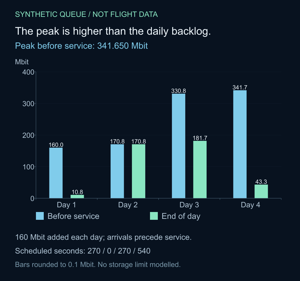
A sequence of contacts reveals problems that a daily average can miss. The Python example uses scheduled durations totalling 270, zero, 270 and 540 seconds on four successive days. Each day first adds two eighty-megabit images to an initially empty queue, then removes whatever useful service is available. The calculated end-of-day backlogs are 10.825, 170.825, 181.650 and 43.300 megabits. A stronger fourth day reduces the queue but does not eliminate it.
This model deliberately aggregates each day's contacts after that day's acquisitions. In that ordering, the largest queue before service is 341.650 megabits, at the start of the fourth day's service. That is higher than any end-of-day value. A storage decision based only on the largest printed final backlog would miss this within-day peak. The diagram distinguishes both quantities so the ordering assumption is visible rather than hidden in a formula.
For a mission study, replace daily buckets with a time-ordered event sequence containing individual acquisitions, transfers and interruptions. Preserve unsuccessful contacts rather than silently redistributing their capacity to another day. Include reserved memory and file-system behaviour, and define what happens when space becomes scarce. The model below has unlimited storage, no deliberate data discard and no acquisition rejection. Its numbers demonstrate queue arithmetic; they do not establish a safe memory capacity or an actual contact plan.
# Invented scenario; SI megabit = 1_000_000 bits.
frame_bits = 1000 * 1000 * 5 * 16
frames_per_day = 2
rate_bps = 1_000_000  # after coding, before file/protocol overhead
usable_time_fraction = 0.65
file_efficiency = 0.85
scheduled_seconds = [270, 0, 270, 540]
backlog = 0.0
peak = 0.0
for day, seconds in enumerate(scheduled_seconds, 1):
    backlog += frames_per_day * frame_bits
    peak = max(peak, backlog)  # arrivals before service in this toy model
    capacity = rate_bps * seconds * usable_time_fraction * file_efficiency
    delivered = min(backlog, capacity)
    backlog -= delivered
    print(f"Day {day}: backlog={backlog / 1e6:.3f} Mbit")
print(f"Peak before service={peak / 1e6:.3f} Mbit")
# Day 1: backlog=10.825 Mbit
# Day 2: backlog=170.825 Mbit
# Day 3: backlog=181.650 Mbit
# Day 4: backlog=43.300 Mbit
# Peak before service=341.650 Mbit
Keep the data budget separate from the radio link budget
NASA's ground-systems chapter describes a link budget as an assessment of end-to-end communication performance, accounting for gains, losses and required margin. It also frames the ground segment as the path from the spacecraft to the end user. The queue calculation answers a narrower question: if an assumed useful service is available at specified times, how much data remains? Passing that arithmetic check is necessary for the chosen scenario, but it cannot prove radio coverage, ground-station booking or successful reception. [2]
Treat the assumptions as a set that must eventually agree with other analyses. Contact timing comes from the chosen orbit and ground assets; available transfer time also competes with spacecraft operations. The achievable rate must agree with the communication analysis, while sustained processing and transmission must agree with power and thermal constraints. Replacing one optimistic input with a supported value may change several others. Record those dependencies so a revised design does not preserve an obsolete capacity estimate by accident.
Budget for scientific usefulness and delivery time
Data volume and scientific usefulness are related but different. A cloudy agricultural frame may still occupy memory and downlink capacity even if ground processing later rejects it. Do not reduce generated volume by an assumed clear-sky fraction unless an actual onboard selection process exists and its behaviour has been evaluated. If selection is proposed, retain the evidence needed to understand false rejections and the observations that never reach the ground. A smaller transfer is not automatically a better scientific service.
Track latency as well as backlog: acquisition time, successful file completion, processing completion and product release can be different events. A partially delivered image is not the same as a verified analysis-ready observation. For BhumiSat's concept research, the next useful step is a traceable scenario sheet connecting sample volume, measured or justified encoding assumptions, event-based service and application deadlines. That provides concrete questions for future payload and ground-system studies while keeping unconfirmed spacecraft capabilities clearly separate from demonstrated results.
Sources & further reading
Explore the engineering questions behind BhumiSat's 2030 vision, revisit multispectral sensor concepts, or connect delivered imagery to field-to-pixel validation.