Comparisons through time are valuable only when the observations are sufficiently comparable for the question being asked. A difference between dates can reflect real change, a normal stage in a seasonal cycle, or a difference in how the surface was observed. This perspective examines the reference period, the timing of acquisitions, and the contextual records needed to interpret a sequence. It encourages the use of appropriate baselines rather than treating every previous observation as an equivalent benchmark. The objective is to identify changes that remain meaningful after normal variation and measurement conditions are considered.
This working guide considers radiometric calibration and reflectance consistency along changing sandy shorelines. The immediate decision is to review shoreline positions over time. Useful reference evidence includes acquisition context, field positions and consistent shoreline definitions. The case is an illustrative planning context, with assumptions to check against the actual sensor, landscape and project requirements.
Define the quantity that the instrument records
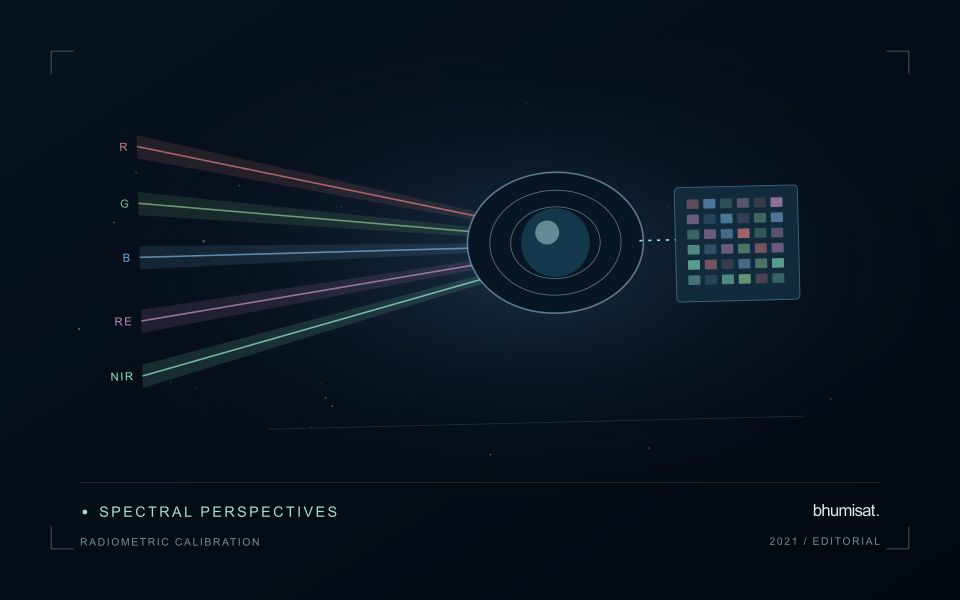
Radiometric calibration establishes a documented relationship between an instrument's recorded output and the physical quantity it is intended to represent. A stored pixel value may be a digital number, a scaled radiance or reflectance value, or another processed representation. Those alternatives should not be treated as interchangeable. The calibration chain explains how the recorded signal becomes an interpretable measurement and which corrections have already been applied. Understanding that chain is essential before comparing dates, combining bands or transferring a model between instruments.
Instrument response can vary across detectors, channels and operating conditions. Calibration therefore concerns more than selecting one conversion coefficient. A study may need to consider offsets, response differences, noise, saturation and changes in behaviour over time. The appropriate characterisation depends on the instrument and its intended use. For a future payload concept, these are requirements to investigate rather than capabilities established by an attractive render. The presence of a multispectral camera alone does not demonstrate that its channels produce consistent, quantitatively comparable observations.
Track consistency through the complete chain
At the product level, begin with the supplier's definitions and metadata. Check scale factors, additive offsets, fill values and valid ranges before deriving an index or statistical summary. Preserve the processing version so that an output can be reproduced later. Inspect whether extreme values correspond to real surfaces or to invalid observations. When a dataset is updated, compare representative old and new results rather than assuming that a familiar file name guarantees an unchanged numerical meaning throughout the archive.
Validation should cover the full chain that supports the stated application. A stable response in a laboratory test is valuable evidence, while operational imagery introduces additional effects from atmosphere, geometry and scene complexity. Use independent references suited to the measurement scale and report the relevant uncertainty. Maintain a record of corrections and their limitations when delivering results to users. A traceable radiometric workflow supports meaningful comparisons and helps separate a change in the observation system from a change in the landscape that a monitoring service is trying to describe.
The setting: Changing sandy shorelines
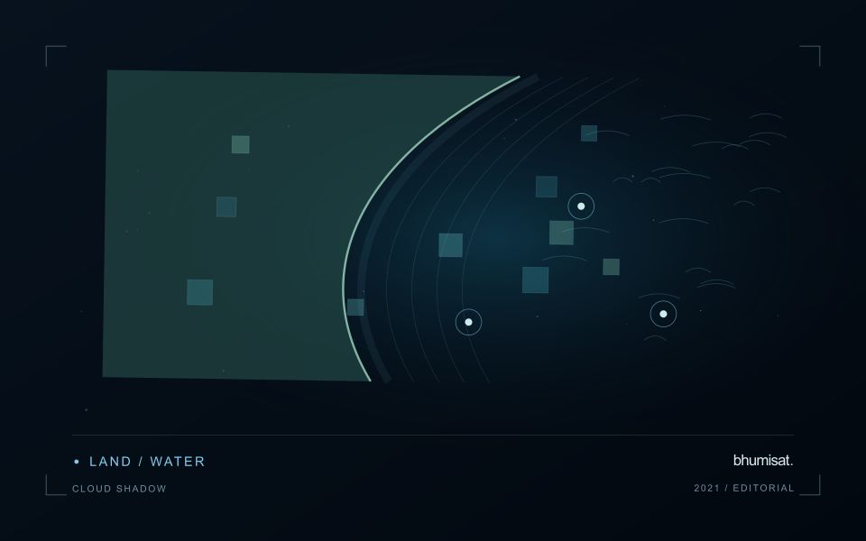
A shoreline is not always one fixed boundary that every observation measures in the same way. The visible water edge, a vegetation boundary and another mapped coastal indicator can represent different features. A monitoring programme should define its chosen shoreline consistently before comparing dates. Tidal conditions, wave state, seasonal beach changes and the geometry of the image can all influence the position recorded, even without a lasting change in the coast.
Spatial resolution and alignment determine the precision with which a boundary can be located. A sharply drawn line on a map should not imply more positional certainty than the observations support. Compare acquisitions under suitable conditions and retain the information needed to examine their differences. Mixed pixels, shadows and narrow coastal features may require manual review or an uncertainty zone rather than an automatic interpretation at every location.
Field validation should use the same shoreline definition as the image analysis and record when and how a position was measured. A visit under different water conditions may represent a different boundary even if its coordinates are accurate. Evaluate change over appropriate distances and periods, and avoid treating every small mapped displacement as erosion or deposition. A transparent product shows the observed positions, their dates and the uncertainty relevant to the decision being considered.
Represent gaps without inventing observations
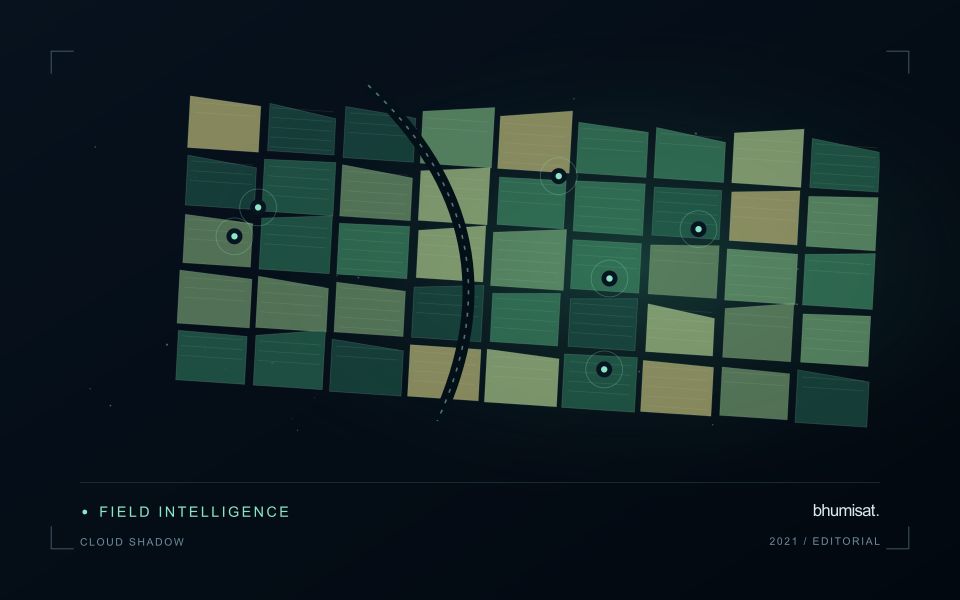
A monitoring sequence often contains periods without a usable observation. The reason may be cloud, shadow, missing coverage, a failed transfer, or a quality condition that excludes the data. Begin by representing these states explicitly. A missing observation is different from a low measurement, an unchanged surface, or a confirmed absence of the feature being studied. The distinction should survive both the analysis and the presentation of the result.
Define when a temporal gap is acceptable for the intended decision. A workflow may continue using the latest qualified observation, request another source, or suspend an alert until sufficient evidence is available. Whichever response is selected, show the age of the supporting observation. If interpolation is used for a suitable analytical purpose, preserve the distinction between an estimated value and a directly observed measurement, together with the assumptions needed to interpret it.
Review how gaps affect the coverage of the final evaluation. Locations with frequent missing data may differ systematically from those with regular observations. A performance estimate based only on clear, complete records can therefore describe a narrower population than the service is expected to support. Report usable coverage alongside analytical results and use recurring gaps to guide acquisition planning, reference collection, and the selection of complementary observation methods.
Design an evaluation that reflects deployment
A model evaluation should resemble the conditions in which the model will be used. Start by identifying which relationships the development data share: nearby locations, repeated observations of the same unit, common collection teams, or measurements from a single period. These relationships can make records less independent than they appear. An evaluation that ignores them may test the ability to recognise familiar conditions rather than the ability to operate in a new setting.
Choose a split strategy that matches the intended transfer. Holding out locations, seasons, operational units, or acquisition conditions can answer different questions. Document which question each split is designed to address, and keep the held-out evidence separate while selecting features and tuning the method. Repeatedly inspecting the same evaluation set to improve a model gradually makes that set part of development, even if it retains its original label.
Report results at a scale that is meaningful to the user. A strong average can hide poor performance for important subgroups or unusual conditions. Examine error patterns and retain examples of both successful and unsuccessful predictions. Where the evidence covers only a limited range of conditions, describe that range explicitly. The evaluation then becomes a practical guide to suitable use, further testing, and the collection of additional reference observations.
Bring the evidence back to the decision
A useful comparison preserves the dates, quality conditions, and contextual assumptions behind its baseline. Review unusual results against the actual observation sequence rather than relying entirely on a summary statistic. Where seasonal timing is important, describe how comparable stages were identified. The resulting analysis should help users distinguish an informative change from an expected cycle or an observation artefact, while making gaps and remaining uncertainty visible enough to guide further investigation.
Sources & further reading
Explore the bhumisat spacecraft concept and our vision towards 2030, or return to the journal.