Comparisons through time are valuable only when the observations are sufficiently comparable for the question being asked. A difference between dates can reflect real change, a normal stage in a seasonal cycle, or a difference in how the surface was observed. This perspective examines the reference period, the timing of acquisitions, and the contextual records needed to interpret a sequence. It encourages the use of appropriate baselines rather than treating every previous observation as an equivalent benchmark. The objective is to identify changes that remain meaningful after normal variation and measurement conditions are considered.
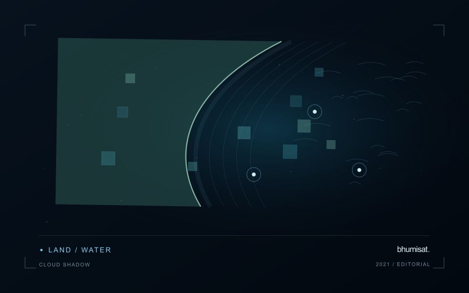
This working guide considers cloud and shadow screening for optical imagery in turbid coastal waters. The immediate decision is to identify coastal sampling priorities. Useful reference evidence includes water samples, surface conditions and acquisition-time context. The case is an illustrative planning context, with assumptions to check against the actual sensor, landscape and project requirements.
The setting: Turbid coastal waters
Turbid coastal waters contain changing mixtures of suspended material, dissolved substances, biological components and surface reflections. Their image appearance may vary over short distances and between acquisitions. A monitoring design should identify which variable or pattern it aims to investigate rather than treating every colour difference as a direct water-quality measurement. Coastal geometry and the proximity of land also influence which parts of an image provide a defensible observation of water.
Review atmospheric conditions, cloud, shadow, sun glint and land adjacency before comparing spectral measurements. Shallow-bottom contributions can matter in some places, while deeper areas may present a different interpretation problem. A relationship developed for one water type should not be transferred automatically to another. Retain the valid observation mask and the dates supporting each map so that users can distinguish measured patterns from periods without suitable optical evidence.
Field validation should sample the range of conditions in which a model or interpretation rule will operate. Record collection time, location and the measurement method for the target variable, together with relevant surface conditions. Samples and imagery separated by a changing coastal event may not be comparable. A useful product can guide sampling or describe a consistent spectral pattern, with stronger numerical water-quality claims introduced only when their calibration and independent evaluation support the intended application.
A quality mask changes the evidence available
Clouds and their shadows can produce strong changes in optical imagery that have little to do with the condition of the land beneath them. A quality mask identifies observations that should be excluded or treated cautiously for a particular analysis. It is not simply a cosmetic step used to improve an image. The mask determines which measurements contribute to an index, field statistic or time-series model. Its assumptions therefore belong in the analytical record and should remain available when a result is reviewed.
A scene with a low overall cloud percentage can still be unsuitable for a particular farm. Conversely, a partly cloudy scene may contain useful observations over the target fields. Evaluate quality at the area of interest rather than relying only on scene-level metadata. Cloud edges, haze and shadow boundaries can be difficult to classify consistently. Depending on the application, an additional exclusion around a flagged feature may be appropriate. The effect of that choice on usable coverage should be measured instead of hidden.
Check the mask as part of the result
Inspect representative successful and unsuccessful cases before adopting a mask rule across a large archive. Check whether bright soil, roofs, water or dark vegetation are being confused with cloud or shadow. Compare automatic flags with image context and, where available, independent observations. A mask that removes too much valid data can be harmful, while one that retains contamination can create false alerts. The acceptable balance depends on the downstream task and the costs of missed observations and misleading interpretations.
Each delivered field result should state the acquisition date and the fraction of the relevant area supported by valid measurements. If too little remains, a missing result can be more informative than a precise-looking number based on an unrepresentative fragment. Keep observation gaps visible in charts and maps. When the masking method or product version changes, assess how the update affects historical comparability. Treating cloud and shadow screening as part of the evidence chain makes the final agricultural or environmental interpretation easier to audit and more dependable in practice.
Establish a metadata contract
Define a small set of metadata that every observation and derived product must carry through the workflow. Useful fields include a stable identifier, acquisition time, geographic reference, spatial coverage, measurement units, source version, and processing status. The purpose is not to collect every possible detail. It is to preserve the information required to interpret, compare, locate, and reproduce the observations that the application depends on.
Specify field names, allowed formats, and the meaning of missing values. A blank field, a value of zero, and a measurement below a detection threshold are different states and should remain distinguishable. Time zones, coordinate order, and unit conversions deserve particular attention because inconsistent conventions can produce plausible-looking results that are difficult to diagnose. Validate the metadata when information enters the system, while the source and collection context remain available.
Treat the metadata contract as part of the delivery interface. A product passed to another team should retain the identifiers needed to trace its source and processing history. If a transformation changes the meaning of a field, create a new field or document the change rather than reusing the original name silently. A clear contract reduces ambiguity between field collectors, analysts, software components, and the eventual users of the information.
Maintain the geographic units of analysis
Many observation services summarise measurements within a field, management block, catchment, forest unit, or other mapped boundary. The meaning of that summary depends on whether the boundary accurately represents the unit being discussed. Start with a clear source for the geometry and record its date, coordinate reference, and intended use. A boundary drawn for visual orientation may require additional checking before it becomes a measurement unit.
Inspect overlaps, gaps, narrow fragments, and features that may have changed since mapping. A geometrically valid polygon can still describe an outdated operational unit. Ask the responsible team how divisions, mergers, new infrastructure, and management changes are recorded. Where pixels or reference measurements cross a boundary, define how they are assigned or excluded so that results remain comparable between analysts and processing runs.
Version the boundaries alongside the observations. If a unit changes, preserve a relationship between the previous and revised geometry rather than replacing the history without explanation. Comparisons through time should identify whether they use a constant spatial unit or the operational units valid at each date. This makes it easier to distinguish a change in the measured surface from a change introduced by the geography used to summarise it.
Bring the evidence back to the decision
A useful comparison preserves the dates, quality conditions, and contextual assumptions behind its baseline. Review unusual results against the actual observation sequence rather than relying entirely on a summary statistic. Where seasonal timing is important, describe how comparable stages were identified. The resulting analysis should help users distinguish an informative change from an expected cycle or an observation artefact, while making gaps and remaining uncertainty visible enough to guide further investigation.
Sources & further reading
Explore the bhumisat spacecraft concept and our vision towards 2030, or return to the journal.