Comparisons through time are valuable only when the observations are sufficiently comparable for the question being asked. A difference between dates can reflect real change, a normal stage in a seasonal cycle, or a difference in how the surface was observed. This perspective examines the reference period, the timing of acquisitions, and the contextual records needed to interpret a sequence. It encourages the use of appropriate baselines rather than treating every previous observation as an equivalent benchmark. The objective is to identify changes that remain meaningful after normal variation and measurement conditions are considered.
This working guide considers rgb satellite imagery for field interpretation across estuarine mixing zones. The immediate decision is to plan sampling across estuarine gradients. Useful reference evidence includes tidal stage, sample timing and water-variable measurements. The case is an illustrative planning context, with assumptions to check against the actual sensor, landscape and project requirements.
The setting: Estuarine mixing zones
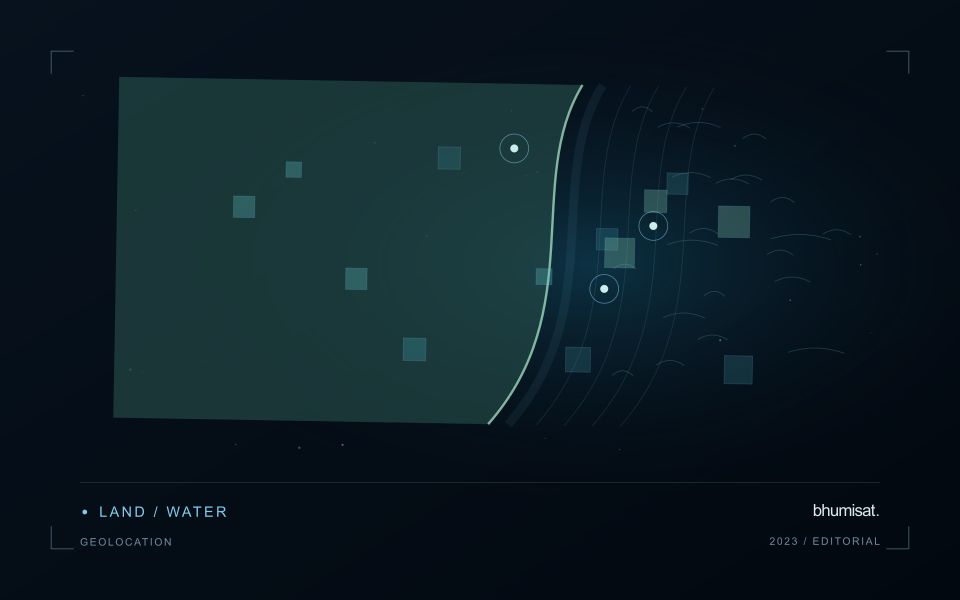
An estuary connects river inflow, coastal water, tidal conditions and complex shorelines. The resulting image pattern may change even when a monitoring team has not altered its methods. A useful design begins with a specific question, such as mapping visible water or investigating a persistent spectral gradient. It should not assume that one relationship describes every part of the estuary or that a single acquisition represents conditions throughout a tidal cycle.
Comparison units should account for channels, shallow margins and locations where land and water are mixed within an observation. Review cloud and atmospheric quality, surface reflection and geometric alignment before interpreting a difference between dates. Tidal and inflow context can help explain the setting but does not replace measurements of the target variable. Preserve the acquisition times and valid areas so that a mapped feature can be evaluated against the conditions under which it was observed.
A validation plan should represent different water types and spatial positions across the mixing zone. Collect the timing and location of samples consistently, and consider whether conditions changed between sampling and acquisition. A spectral boundary may help organise an investigation without proving a particular source or ecological consequence. More specific interpretations require evidence designed for those claims, while an auditable record of observed patterns and sampling priorities can already improve the structure of a monitoring programme.
Use visible context carefully
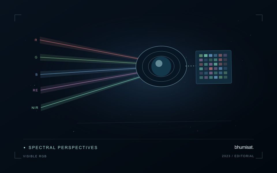
A familiar colour image combines red, green and blue measurements into a display that resembles human visual experience. That familiarity helps people recognise fields, roads, exposed soil, water and settlement patterns. It can also create a false sense that interpretation is effortless. Satellite imagery is influenced by acquisition conditions, processing and display choices. The image may not show the same colours an observer would have seen from the ground. Its value lies in spatial context, supported by a clear account of how the display was produced.
Contrast stretching makes subtle patterns easier to see, but it can make two dates look different even when the underlying reflectance is similar. An automatic stretch selected separately for each image is useful for exploration and less suitable as evidence of a measured change. Keep acquisition dates visible and distinguish a display adjustment from an analytical transformation. When comparing scenes, use a consistent viewing approach and inspect the original values or a suitable quantitative product before drawing a conclusion from colour alone.
Prepare a repeatable visual review
Visible imagery supports a practical first review of a monitoring result. Check whether a field boundary follows the current cultivated area and whether paths, buildings or neighbouring vegetation are included accidentally. Look for management changes that may explain a spectral anomaly, such as harvest, replanting or newly exposed ground. A visual check can identify a plausible explanation and guide field inspection. It should not be presented as proof of a specific disease, nutrient deficiency or production outcome without evidence suited to that claim.
A repeatable review protocol records what the analyst examined and how confidently it could be interpreted. The record can include cloud and shadow presence, obvious mapping errors, the age of the image and any feature requiring confirmation. Use agreed descriptions so that different reviewers can compare their findings. Where a detail is smaller than the available spatial information, acknowledge that limitation and seek a complementary observation. RGB imagery is a useful interface between technical analysis and field knowledge when its visual clarity is accompanied by disciplined interpretation.
Deliver quality flags that users can interpret
Quality information should describe the condition of an observation in terms that remain useful through the workflow. A single valid or invalid label may be sufficient for some calculations, but operational users often need to know why an observation was qualified. Distinguish acquisition limitations, processing failures, uncertain reference matches, and conditions that make interpretation ambiguous. These categories point towards different responses and should not be merged without a clear purpose.
Define a small, documented set of flags with stable meanings. Record whether a flag applies to a complete scene, a geographic unit, an individual measurement, or a derived result. A unit containing a mixture of qualified and unqualified observations may also require a coverage measure. Include the rule used to combine flags when summarising data so that a favourable average does not conceal a substantial fraction of unusable input.
Test the flags with the people receiving the product. Ask what they would do differently for each state and whether the terminology supports that choice. Keep the original flags available even if the interface presents a simpler summary. When flag definitions change, version the rules and review their effects on historical comparisons. Useful quality communication makes the condition of the evidence visible at the moment when a user decides how much confidence to place in the result.
Represent gaps without inventing observations
A monitoring sequence often contains periods without a usable observation. The reason may be cloud, shadow, missing coverage, a failed transfer, or a quality condition that excludes the data. Begin by representing these states explicitly. A missing observation is different from a low measurement, an unchanged surface, or a confirmed absence of the feature being studied. The distinction should survive both the analysis and the presentation of the result.
Define when a temporal gap is acceptable for the intended decision. A workflow may continue using the latest qualified observation, request another source, or suspend an alert until sufficient evidence is available. Whichever response is selected, show the age of the supporting observation. If interpolation is used for a suitable analytical purpose, preserve the distinction between an estimated value and a directly observed measurement, together with the assumptions needed to interpret it.
Review how gaps affect the coverage of the final evaluation. Locations with frequent missing data may differ systematically from those with regular observations. A performance estimate based only on clear, complete records can therefore describe a narrower population than the service is expected to support. Report usable coverage alongside analytical results and use recurring gaps to guide acquisition planning, reference collection, and the selection of complementary observation methods.
Bring the evidence back to the decision
A useful comparison preserves the dates, quality conditions, and contextual assumptions behind its baseline. Review unusual results against the actual observation sequence rather than relying entirely on a summary statistic. Where seasonal timing is important, describe how comparable stages were identified. The resulting analysis should help users distinguish an informative change from an expected cycle or an observation artefact, while making gaps and remaining uncertainty visible enough to guide further investigation.
Sources & further reading
Explore the bhumisat spacecraft concept and our vision towards 2030, or return to the journal.