Comparisons through time are valuable only when the observations are sufficiently comparable for the question being asked. A difference between dates can reflect real change, a normal stage in a seasonal cycle, or a difference in how the surface was observed. This perspective examines the reference period, the timing of acquisitions, and the contextual records needed to interpret a sequence. It encourages the use of appropriate baselines rather than treating every previous observation as an equivalent benchmark. The objective is to identify changes that remain meaningful after normal variation and measurement conditions are considered.
This working guide considers building a spacecraft power and energy budget in seasonal dry woodlands. The immediate decision is to distinguish seasonal change from disturbance. Useful reference evidence includes leafing stage, disturbance evidence and land-management records. The case is an illustrative planning context, with assumptions to check against the actual sensor, landscape and project requirements.
Distinguish power from stored energy
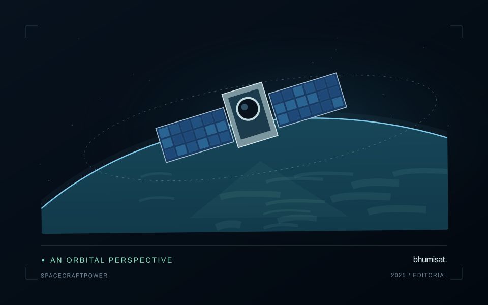
A spacecraft electrical power system must generate energy, store it when necessary and distribute it reliably to the loads. Power describes the rate of energy use, while energy describes consumption over an interval. A transmitter may have a high instantaneous demand even if it operates briefly. Conversely, a modest continuous load can dominate the daily energy budget. Both views are needed to size the system.
List operating modes and their duration: standby, imaging, processing, communication, safe mode and any relevant transitions. Include heaters, power conversion losses and supporting electronics rather than counting only the camera and radio. Identify loads that overlap in time and those that can be scheduled separately. Peak current and startup behavior can challenge distribution hardware even when the average energy balance appears comfortable.
Check realistic orbit and lifetime conditions
Solar generation depends on illumination, array orientation, temperature and the condition of the cells and associated hardware. Eclipse intervals require stored energy, and imaging or communication pointing may reduce favorable Sun exposure. Evaluate the time sequence across representative orbits rather than comparing one average generation number with one average load. Consider the expected decline in performance over the mission and apply clearly justified design margins.
Battery sizing must consider usable capacity under the planned temperature, discharge rate and cycling conditions. Nominal capacity alone does not describe what is safely available in service. Charging limits, allowed depth of discharge, ageing and monitoring requirements influence the operating envelope. Thermal design and power planning therefore need to evolve together. A heater can protect a battery while consuming the energy that the battery is expected to deliver.
The distribution system should detect and isolate relevant faults while preserving essential functions. Define which loads are shed when energy becomes scarce and what conditions allow them to return. Safe mode needs its own verified energy balance and a credible path toward recovery. Telemetry should support comparison between predicted and measured generation, consumption and battery behavior. Test the budget with realistic duty cycles, instrument startup sequences and communication sessions, then update the model using measured component performance. A defensible power plan explains the worst cases and the assumptions behind its reserve, allowing observation schedules to be adjusted before they threaten spacecraft survival.
The setting: Seasonal dry woodlands
Seasonal dry woodlands can change markedly in appearance as leaf cover, understory vegetation and soil exposure vary through the year. A sparse-looking canopy during one period may be part of an ordinary seasonal cycle rather than evidence of degradation. Interpretation should begin with the local seasonal context and the intended observation variable. Mapping woody cover, reviewing a disturbance alert and studying vegetation recovery require related but distinct forms of evidence.
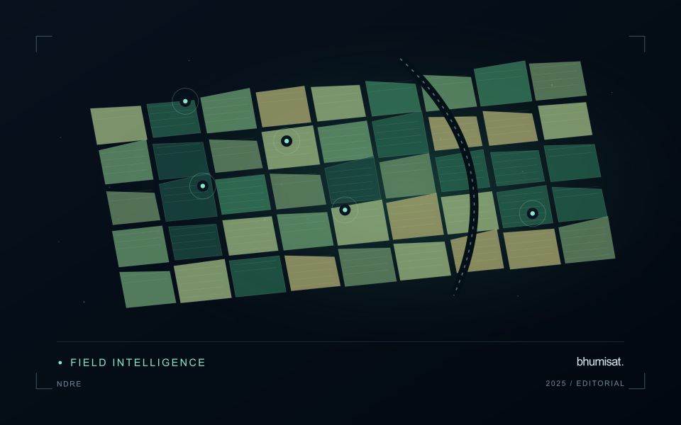
Build comparisons using appropriate dates and quality-screened measurements, and examine whether an apparent change persists beyond a short seasonal fluctuation. Ground vegetation can contribute strongly where tree cover is open. Rainfall timing, grazing or other land management may alter that contribution without changing the woody component. A report should retain the observed area and acquisition dates so that a user can distinguish a current measurement from an inference made across a long image gap.
Field validation should record tree and ground-layer conditions separately where that distinction matters to the application. Include the leafing stage, signs of recent disturbance and the management context of each sampled area. A decline in a vegetation measure cannot identify its cause by itself. Evaluate mapped changes against representative observations across different canopy densities and seasonal states, and communicate where the available imagery supports a broad landscape interpretation rather than a precise inventory of individual trees.
Prioritise observations within delivery constraints
An observation has practical value only if it can reach the processing and user workflow in a suitable form and time. Delivery planning therefore belongs alongside acquisition planning. Identify the volume and priority of expected data, the opportunities available for transfer, and the consequences of delay. A system may collect more information than it can deliver promptly, so the handling of that difference should be an explicit design choice.
Define priorities using the information need rather than only the order in which files were created. A small set of timely, qualified observations may support a decision more effectively than a larger volume delivered after the relevant opportunity has passed. Preserve enough metadata to recognise each observation and its completeness during transfer. If compression, reduced products, or staged delivery are considered, evaluate how those choices affect the interpretation and subsequent processing of the information.
Test the delivery sequence with representative conditions, including interruptions and incomplete transfers. Establish how the receiving system verifies integrity, identifies missing components, and requests or schedules recovery where that is supported. Keep a record of actual delivery age and usable coverage. For a mission concept, these tests can be performed with simulated data flows before an operational claim is made. The objective is a delivery plan whose constraints are visible in the service that users receive.
Check spatial alignment before comparison
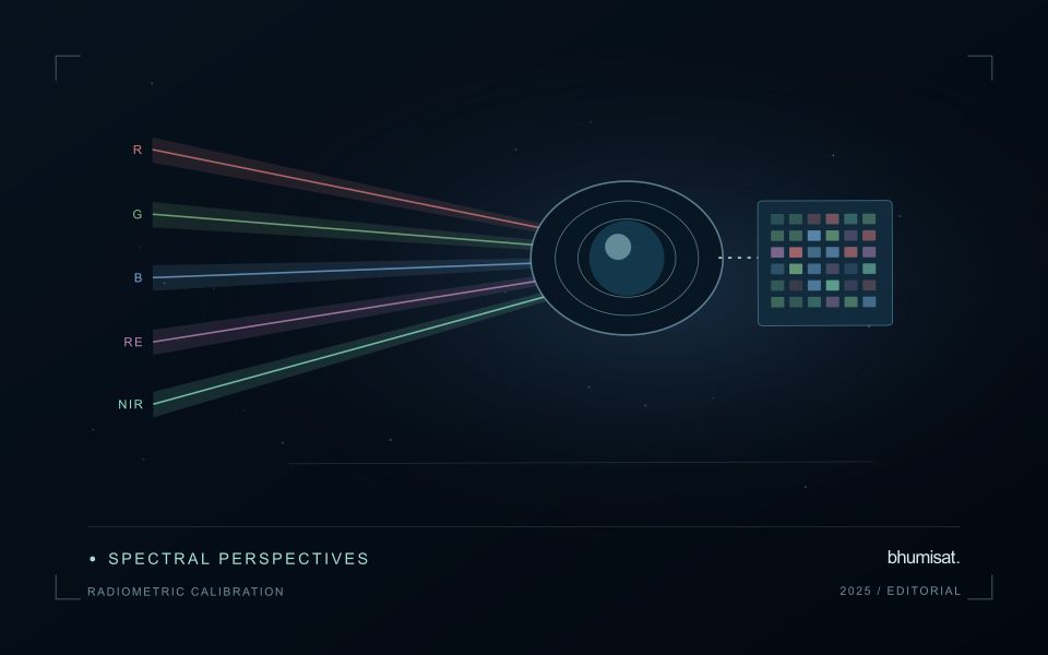
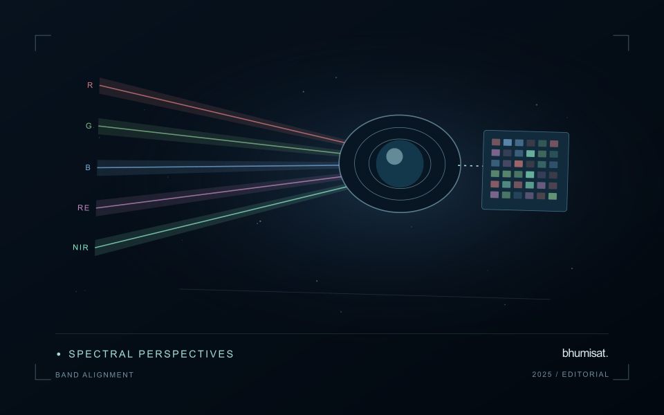
A comparison between images, channels, maps, or field measurements assumes that the observations refer to the same locations at a suitable level of precision. Small alignment errors can become especially important near boundaries or narrow features. Before interpreting differences, inspect whether identifiable, stable features agree between the sources. A common coordinate reference is necessary for many workflows, but it does not by itself demonstrate accurate alignment.
Use control features that are appropriate for the observation scale and remain stable across the comparison period. Evaluate alignment in more than one part of the area, because a single location cannot reveal spatially varying distortion. Record the method used to estimate any correction and retain independent features for checking the corrected result. Where surfaces have genuinely changed, avoid using those changes as evidence of an alignment error.
Propagate the implications of remaining misalignment into the analysis. A workflow may exclude boundary pixels, summarise at a broader scale, or qualify interpretations for small features. The choice should follow the application rather than a preference for visually smooth output. Preserve both the original and corrected geographic references, and document resampling decisions so that future users can understand how measurements were moved onto a common spatial framework.
Bring the evidence back to the decision
A useful comparison preserves the dates, quality conditions, and contextual assumptions behind its baseline. Review unusual results against the actual observation sequence rather than relying entirely on a summary statistic. Where seasonal timing is important, describe how comparable stages were identified. The resulting analysis should help users distinguish an informative change from an expected cycle or an observation artefact, while making gaps and remaining uncertainty visible enough to guide further investigation.
Sources & further reading
Explore the bhumisat spacecraft concept and our vision towards 2030, or return to the journal.