A workflow that succeeds on a small study area may encounter different constraints when the number of observations, locations, or users increases. Scaling requires attention to processing capacity, data organisation, reference coverage, and the effort needed to review results. This perspective looks beyond whether a calculation can run on a larger dataset. It asks whether the complete service can preserve its meaning, quality, and delivery commitments as its scope expands. The objective is a design that identifies bottlenecks early and increases throughput without silently weakening the evidence available to users.
This working guide considers building a spacecraft power and energy budget along changing sandy shorelines. The immediate decision is to review shoreline positions over time. Useful reference evidence includes acquisition context, field positions and consistent shoreline definitions. The case is an illustrative planning context, with assumptions to check against the actual sensor, landscape and project requirements.
Distinguish power from stored energy
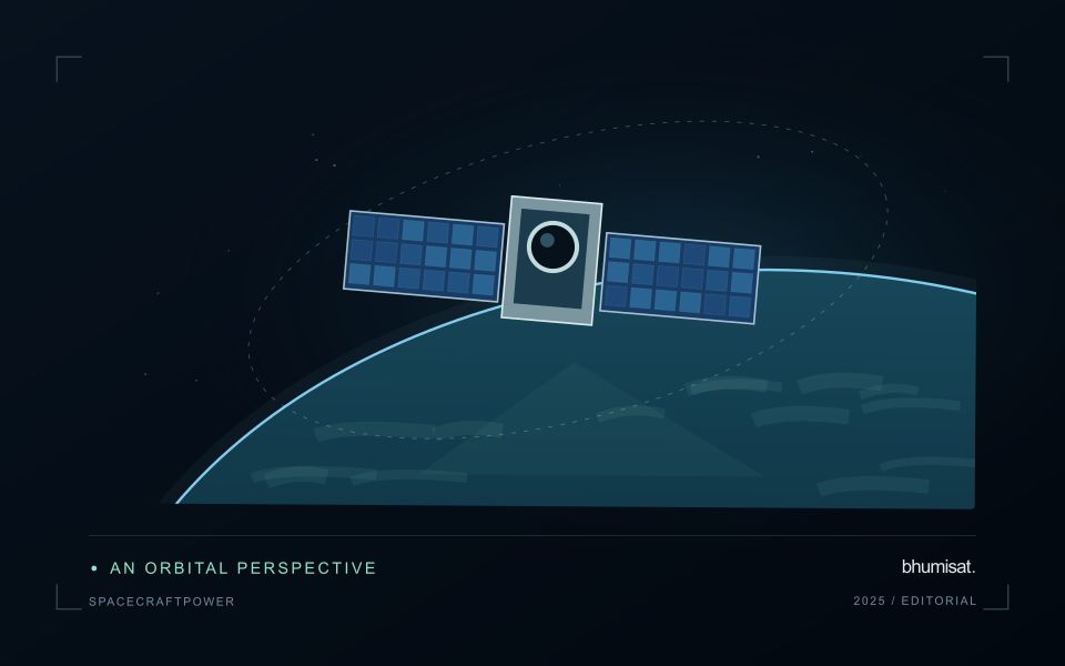
A spacecraft electrical power system must generate energy, store it when necessary and distribute it reliably to the loads. Power describes the rate of energy use, while energy describes consumption over an interval. A transmitter may have a high instantaneous demand even if it operates briefly. Conversely, a modest continuous load can dominate the daily energy budget. Both views are needed to size the system.
List operating modes and their duration: standby, imaging, processing, communication, safe mode and any relevant transitions. Include heaters, power conversion losses and supporting electronics rather than counting only the camera and radio. Identify loads that overlap in time and those that can be scheduled separately. Peak current and startup behavior can challenge distribution hardware even when the average energy balance appears comfortable.
Check realistic orbit and lifetime conditions
Solar generation depends on illumination, array orientation, temperature and the condition of the cells and associated hardware. Eclipse intervals require stored energy, and imaging or communication pointing may reduce favorable Sun exposure. Evaluate the time sequence across representative orbits rather than comparing one average generation number with one average load. Consider the expected decline in performance over the mission and apply clearly justified design margins.
Battery sizing must consider usable capacity under the planned temperature, discharge rate and cycling conditions. Nominal capacity alone does not describe what is safely available in service. Charging limits, allowed depth of discharge, ageing and monitoring requirements influence the operating envelope. Thermal design and power planning therefore need to evolve together. A heater can protect a battery while consuming the energy that the battery is expected to deliver.
The distribution system should detect and isolate relevant faults while preserving essential functions. Define which loads are shed when energy becomes scarce and what conditions allow them to return. Safe mode needs its own verified energy balance and a credible path toward recovery. Telemetry should support comparison between predicted and measured generation, consumption and battery behavior. Test the budget with realistic duty cycles, instrument startup sequences and communication sessions, then update the model using measured component performance. A defensible power plan explains the worst cases and the assumptions behind its reserve, allowing observation schedules to be adjusted before they threaten spacecraft survival.
The setting: Changing sandy shorelines
A shoreline is not always one fixed boundary that every observation measures in the same way. The visible water edge, a vegetation boundary and another mapped coastal indicator can represent different features. A monitoring programme should define its chosen shoreline consistently before comparing dates. Tidal conditions, wave state, seasonal beach changes and the geometry of the image can all influence the position recorded, even without a lasting change in the coast.
Spatial resolution and alignment determine the precision with which a boundary can be located. A sharply drawn line on a map should not imply more positional certainty than the observations support. Compare acquisitions under suitable conditions and retain the information needed to examine their differences. Mixed pixels, shadows and narrow coastal features may require manual review or an uncertainty zone rather than an automatic interpretation at every location.
Field validation should use the same shoreline definition as the image analysis and record when and how a position was measured. A visit under different water conditions may represent a different boundary even if its coordinates are accurate. Evaluate change over appropriate distances and periods, and avoid treating every small mapped displacement as erosion or deposition. A transparent product shows the observed positions, their dates and the uncertainty relevant to the decision being considered.
Connect observations within a catchment
Water-related observations often depend on processes beyond the immediate pixel or sampling location. Begin by identifying the geographic relationships that are relevant to the question: upstream areas, connected drainage paths, contributing land uses, and the receiving water body. A local pattern may be easier to interpret when placed within that wider setting. The catchment boundary is a useful organising unit, but its suitability should be checked against the process and observation scale.
Combine the remote observation with contextual records that can help explain its timing and spatial pattern. Rainfall, water level, land management, and known interventions can influence what is observed. Preserve the dates and geographic meaning of those records rather than treating them as timeless attributes. Where drainage connections are uncertain or change with conditions, state the limitation and consider whether additional mapping or reference observations would materially improve the interpretation.
Plan reference sampling across locations that distinguish plausible explanations. A set of measurements concentrated at an easily accessible outlet may provide a different view from one that also represents tributaries, source areas, and contrasting conditions. Document how each location contributes to the evaluation. Interpret spatial agreement with care, because connected observations can share influences and may not provide independent evidence. The resulting workflow should connect local measurements with a defensible account of the wider system they help describe.
Represent gaps without inventing observations
A monitoring sequence often contains periods without a usable observation. The reason may be cloud, shadow, missing coverage, a failed transfer, or a quality condition that excludes the data. Begin by representing these states explicitly. A missing observation is different from a low measurement, an unchanged surface, or a confirmed absence of the feature being studied. The distinction should survive both the analysis and the presentation of the result.
Define when a temporal gap is acceptable for the intended decision. A workflow may continue using the latest qualified observation, request another source, or suspend an alert until sufficient evidence is available. Whichever response is selected, show the age of the supporting observation. If interpolation is used for a suitable analytical purpose, preserve the distinction between an estimated value and a directly observed measurement, together with the assumptions needed to interpret it.
Review how gaps affect the coverage of the final evaluation. Locations with frequent missing data may differ systematically from those with regular observations. A performance estimate based only on clear, complete records can therefore describe a narrower population than the service is expected to support. Report usable coverage alongside analytical results and use recurring gaps to guide acquisition planning, reference collection, and the selection of complementary observation methods.
Bring the evidence back to the decision
Expansion should be guided by measured workload, visible quality conditions, and an understanding of which tasks require expert attention. Test the workflow under representative data volumes before treating a successful demonstration as evidence of operational capacity. Preserve a route for investigating individual observations even when most processing is automated. A scalable service keeps its results traceable and useful as it grows, with clear choices about where to automate, where to review, and where to invest in additional evidence.
Sources & further reading
Explore the bhumisat spacecraft concept and our vision towards 2030, or return to the journal.