Comparisons through time are valuable only when the observations are sufficiently comparable for the question being asked. A difference between dates can reflect real change, a normal stage in a seasonal cycle, or a difference in how the surface was observed. This perspective examines the reference period, the timing of acquisitions, and the contextual records needed to interpret a sequence. It encourages the use of appropriate baselines rather than treating every previous observation as an equivalent benchmark. The objective is to identify changes that remain meaningful after normal variation and measurement conditions are considered.
This working guide considers optical payload choices for small satellites in soybean production fields. The immediate decision is to direct scouting to unusual field zones. Useful reference evidence includes planting dates, canopy closure and crop-stage observations. The case is an illustrative planning context, with assumptions to check against the actual sensor, landscape and project requirements.
The setting: Soybean production fields
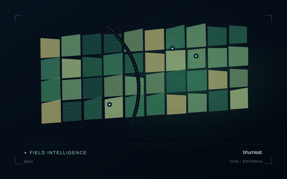
Soybean imagery can show substantial variation as fields progress from exposed soil to closed canopy and eventually to maturity. Planting date, stand arrangement, variety and management can shift that progression. Use these factors to define comparison groups before labelling a field unusual. The boundary dataset should distinguish the planted area from tracks, drainage features and other surfaces that can contribute a large share of the measurement in small or irregular fields.
A practical analytical sequence combines quality-screened imagery with the field calendar and relevant management notes. Review whether an apparent difference persists across usable observations and whether it follows a plausible spatial pattern within the field. An index response can be affected by background soil, weeds, residue or illumination as well as the crop. These possibilities should guide the investigation rather than being collapsed into an automatic claim about plant nutrition or disease.
A field team can test whether the mapped zones correspond to different crop stages or other observable conditions. Collect samples across the range of mapped responses, and include typical areas to avoid evaluating only conspicuous anomalies. Where production estimates are proposed, match the spatial and temporal scale of the reference data to the prediction. A field-average yield record cannot directly validate every small pixel-level variation shown on an attractive map.
Connect the optical design to the measurement
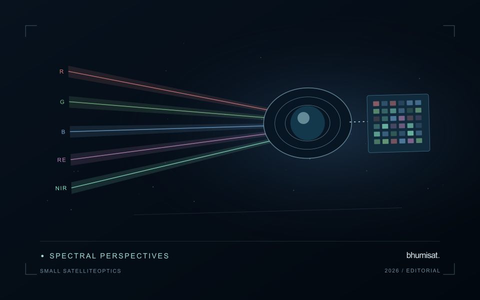
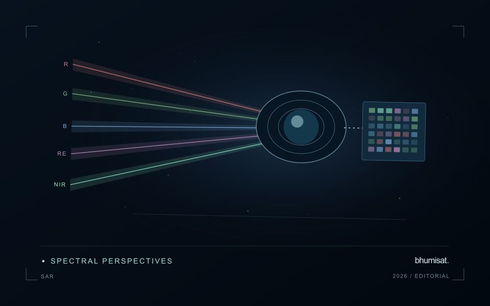
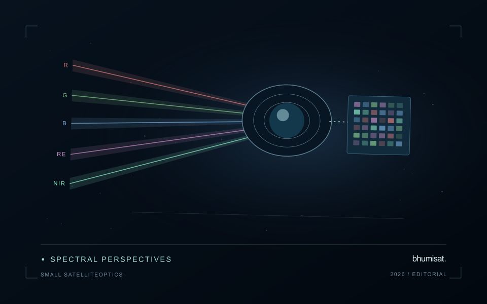
An optical Earth observation payload turns incoming radiance into sampled measurements. Its usefulness depends on more than the ground size represented by a pixel. The aperture, focal length, detector characteristics, spectral response and operating environment all influence the information that survives into the image. A mission should choose these features around a target measurement and its expected brightness, rather than treating pixel spacing as a complete performance specification.
Ground sampling distance describes the spacing of samples on the surface for a specified viewing geometry. Optical blur, detector response, motion and processing can reduce the detail that is actually resolved. The modulation transfer function expresses how contrast is retained across spatial frequencies and helps connect component performance with final image sharpness. Smaller pixels alone cannot recover detail removed by the optical system or excessive image motion.
Balance signal, packaging and calibration
A larger entrance aperture can collect more light, but it also creates demands on mass, volume, alignment and thermal control. Narrow spectral bands collect less energy than broader bands under otherwise comparable conditions. Longer integration can improve signal collection until motion, saturation or other constraints become limiting. The resulting trade must be evaluated for dark targets as well as bright land, and for the expected range of illumination and atmospheric conditions.
Small spacecraft packaging makes mechanical and thermal interfaces particularly consequential. Focus and alignment can shift as temperatures change, while launch loads and contamination can affect performance. Stray light from outside the intended field can bias measurements even when an image appears visually acceptable. Baffles, suitable materials, cleanliness procedures and representative testing help control these effects. Detector defects, nonuniform response and electronic noise also require characterization.
Plan radiometric, geometric and spectral calibration with the payload design. Establish how ground tests connect to measurements after launch, and how changes in response will be monitored. The calibration record should describe uncertainties and conditions, rather than just providing a correction file. Evaluate the complete imaging chain using representative scenes and realistic motion assumptions. A credible specification states where performance is expected, how it will be measured and which tradeoffs were accepted. It should not turn a detector data sheet into an unsupported claim about an entire spacecraft.
Budget the complete processing workflow
A processing budget should cover the complete path from source observations to a maintained product. Data access and computing are only part of that path. Include preparation, geographic updates, reference collection, expert review, delivery, and support where those activities belong to the service. A calculation that runs cheaply on a small demonstration can still require substantial effort when the surrounding work is repeated across many locations.
Measure representative tasks rather than assuming that every observation costs the same amount to process. Record data volume, processing time, retry frequency, manual interventions, and the conditions that create unusually demanding cases. Separate fixed setup work from work that grows with the number of observations or users. These records support decisions about batching, caching, storage policy, and the point at which a different processing design becomes worthwhile.
Connect the budget to a defined level of service. Faster delivery, more frequent observation, broader coverage, or more detailed review can each change the resources required. Describe these trade-offs before promising a delivery pattern that the workflow has not demonstrated. Review the budget using operational evidence and preserve enough detail to understand changes between processing versions. The aim is a sustainable service whose resource choices remain aligned with the information that users value.
Use observation labels with consistent meanings
A reference label should describe an observation that another person could recognise or reproduce. Broad terms such as good, damaged, or unusual can conceal substantial differences between collection teams. Begin by defining the feature or condition being recorded, the observation unit, and the evidence needed to assign a label. Where possible, distinguish a direct measurement from an interpretation made by the observer.
Provide a short collection guide with examples, boundary cases, and a way to record uncertainty. Train observers using shared cases before relying on independently collected labels. If two observers disagree, preserve the disagreement long enough to understand its cause. It may reveal an unclear definition, a genuinely ambiguous condition, a difference in observation scale, or a problem in matching the reference record to the remote measurement.
Retain the context that makes the label interpretable. Location, time, collection method, observer role, and relevant surface conditions can be essential for later review. Changes to the label scheme should be documented and related to earlier versions where a defensible correspondence exists. Consistent labels do not eliminate uncertainty, but they make it possible to investigate disagreement, evaluate analytical methods, and identify where better definitions or additional measurements would improve the evidence.
Bring the evidence back to the decision
A useful comparison preserves the dates, quality conditions, and contextual assumptions behind its baseline. Review unusual results against the actual observation sequence rather than relying entirely on a summary statistic. Where seasonal timing is important, describe how comparable stages were identified. The resulting analysis should help users distinguish an informative change from an expected cycle or an observation artefact, while making gaps and remaining uncertainty visible enough to guide further investigation.
Sources & further reading
Explore the bhumisat spacecraft concept and our vision towards 2030, or return to the journal.