A workflow that succeeds on a small study area may encounter different constraints when the number of observations, locations, or users increases. Scaling requires attention to processing capacity, data organisation, reference coverage, and the effort needed to review results. This perspective looks beyond whether a calculation can run on a larger dataset. It asks whether the complete service can preserve its meaning, quality, and delivery commitments as its scope expands. The objective is a design that identifies bottlenecks early and increases throughput without silently weakening the evidence available to users.
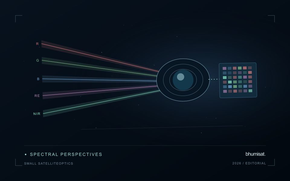
This working guide considers optical payload choices for small satellites in seasonal dry woodlands. The immediate decision is to distinguish seasonal change from disturbance. Useful reference evidence includes leafing stage, disturbance evidence and land-management records. The case is an illustrative planning context, with assumptions to check against the actual sensor, landscape and project requirements.
The setting: Seasonal dry woodlands
Seasonal dry woodlands can change markedly in appearance as leaf cover, understory vegetation and soil exposure vary through the year. A sparse-looking canopy during one period may be part of an ordinary seasonal cycle rather than evidence of degradation. Interpretation should begin with the local seasonal context and the intended observation variable. Mapping woody cover, reviewing a disturbance alert and studying vegetation recovery require related but distinct forms of evidence.
Build comparisons using appropriate dates and quality-screened measurements, and examine whether an apparent change persists beyond a short seasonal fluctuation. Ground vegetation can contribute strongly where tree cover is open. Rainfall timing, grazing or other land management may alter that contribution without changing the woody component. A report should retain the observed area and acquisition dates so that a user can distinguish a current measurement from an inference made across a long image gap.
Field validation should record tree and ground-layer conditions separately where that distinction matters to the application. Include the leafing stage, signs of recent disturbance and the management context of each sampled area. A decline in a vegetation measure cannot identify its cause by itself. Evaluate mapped changes against representative observations across different canopy densities and seasonal states, and communicate where the available imagery supports a broad landscape interpretation rather than a precise inventory of individual trees.
Connect the optical design to the measurement
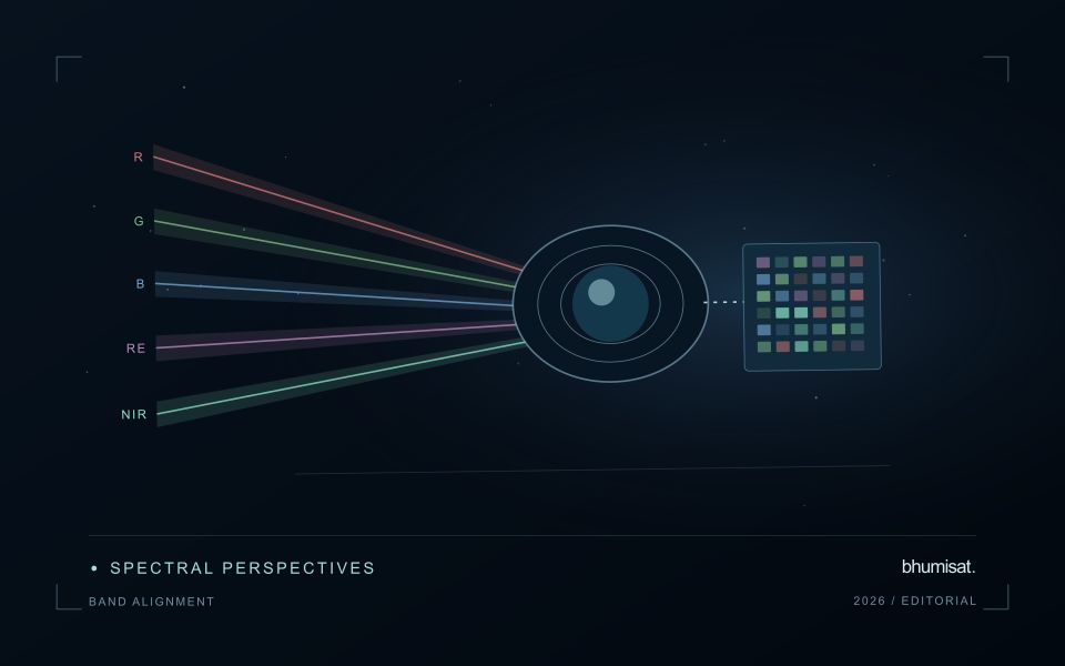
An optical Earth observation payload turns incoming radiance into sampled measurements. Its usefulness depends on more than the ground size represented by a pixel. The aperture, focal length, detector characteristics, spectral response and operating environment all influence the information that survives into the image. A mission should choose these features around a target measurement and its expected brightness, rather than treating pixel spacing as a complete performance specification.
Ground sampling distance describes the spacing of samples on the surface for a specified viewing geometry. Optical blur, detector response, motion and processing can reduce the detail that is actually resolved. The modulation transfer function expresses how contrast is retained across spatial frequencies and helps connect component performance with final image sharpness. Smaller pixels alone cannot recover detail removed by the optical system or excessive image motion.
Balance signal, packaging and calibration
A larger entrance aperture can collect more light, but it also creates demands on mass, volume, alignment and thermal control. Narrow spectral bands collect less energy than broader bands under otherwise comparable conditions. Longer integration can improve signal collection until motion, saturation or other constraints become limiting. The resulting trade must be evaluated for dark targets as well as bright land, and for the expected range of illumination and atmospheric conditions.
Small spacecraft packaging makes mechanical and thermal interfaces particularly consequential. Focus and alignment can shift as temperatures change, while launch loads and contamination can affect performance. Stray light from outside the intended field can bias measurements even when an image appears visually acceptable. Baffles, suitable materials, cleanliness procedures and representative testing help control these effects. Detector defects, nonuniform response and electronic noise also require characterization.
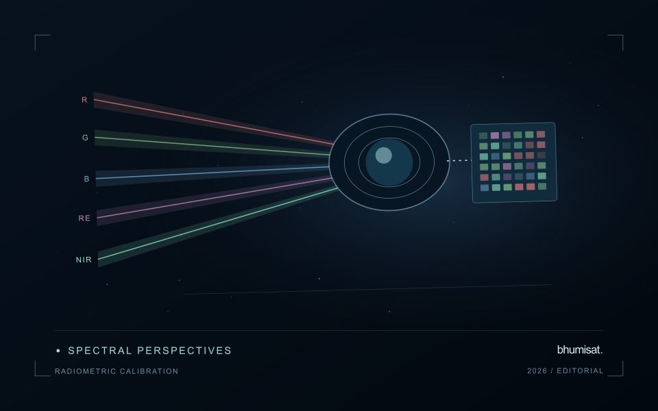
Plan radiometric, geometric and spectral calibration with the payload design. Establish how ground tests connect to measurements after launch, and how changes in response will be monitored. The calibration record should describe uncertainties and conditions, rather than just providing a correction file. Evaluate the complete imaging chain using representative scenes and realistic motion assumptions. A credible specification states where performance is expected, how it will be measured and which tradeoffs were accepted. It should not turn a detector data sheet into an unsupported claim about an entire spacecraft.
Represent gaps without inventing observations
A monitoring sequence often contains periods without a usable observation. The reason may be cloud, shadow, missing coverage, a failed transfer, or a quality condition that excludes the data. Begin by representing these states explicitly. A missing observation is different from a low measurement, an unchanged surface, or a confirmed absence of the feature being studied. The distinction should survive both the analysis and the presentation of the result.
Define when a temporal gap is acceptable for the intended decision. A workflow may continue using the latest qualified observation, request another source, or suspend an alert until sufficient evidence is available. Whichever response is selected, show the age of the supporting observation. If interpolation is used for a suitable analytical purpose, preserve the distinction between an estimated value and a directly observed measurement, together with the assumptions needed to interpret it.
Review how gaps affect the coverage of the final evaluation. Locations with frequent missing data may differ systematically from those with regular observations. A performance estimate based only on clear, complete records can therefore describe a narrower population than the service is expected to support. Report usable coverage alongside analytical results and use recurring gaps to guide acquisition planning, reference collection, and the selection of complementary observation methods.
Deliver quality flags that users can interpret
Quality information should describe the condition of an observation in terms that remain useful through the workflow. A single valid or invalid label may be sufficient for some calculations, but operational users often need to know why an observation was qualified. Distinguish acquisition limitations, processing failures, uncertain reference matches, and conditions that make interpretation ambiguous. These categories point towards different responses and should not be merged without a clear purpose.
Define a small, documented set of flags with stable meanings. Record whether a flag applies to a complete scene, a geographic unit, an individual measurement, or a derived result. A unit containing a mixture of qualified and unqualified observations may also require a coverage measure. Include the rule used to combine flags when summarising data so that a favourable average does not conceal a substantial fraction of unusable input.
Test the flags with the people receiving the product. Ask what they would do differently for each state and whether the terminology supports that choice. Keep the original flags available even if the interface presents a simpler summary. When flag definitions change, version the rules and review their effects on historical comparisons. Useful quality communication makes the condition of the evidence visible at the moment when a user decides how much confidence to place in the result.
Bring the evidence back to the decision
Expansion should be guided by measured workload, visible quality conditions, and an understanding of which tasks require expert attention. Test the workflow under representative data volumes before treating a successful demonstration as evidence of operational capacity. Preserve a route for investigating individual observations even when most processing is automated. A scalable service keeps its results traceable and useful as it grows, with clear choices about where to automate, where to review, and where to invest in additional evidence.
Sources & further reading
Explore the bhumisat spacecraft concept and our vision towards 2030, or return to the journal.