Every observation and interpretation contains uncertainty, but the sources and consequences of that uncertainty differ between applications. Some arise from acquisition conditions, others from reference measurements, processing choices, or the transfer of a model to a new setting. This perspective examines how those sources affect the decision a user is considering. It encourages teams to describe uncertainty in a form that can influence action, rather than adding a generic qualification at the end of a report. The objective is to support proportionate decisions while keeping the limits of the available evidence understandable.
This working guide considers optical payload choices for small satellites across estuarine mixing zones. The immediate decision is to plan sampling across estuarine gradients. Useful reference evidence includes tidal stage, sample timing and water-variable measurements. The case is an illustrative planning context, with assumptions to check against the actual sensor, landscape and project requirements.
The setting: Estuarine mixing zones
An estuary connects river inflow, coastal water, tidal conditions and complex shorelines. The resulting image pattern may change even when a monitoring team has not altered its methods. A useful design begins with a specific question, such as mapping visible water or investigating a persistent spectral gradient. It should not assume that one relationship describes every part of the estuary or that a single acquisition represents conditions throughout a tidal cycle.
Comparison units should account for channels, shallow margins and locations where land and water are mixed within an observation. Review cloud and atmospheric quality, surface reflection and geometric alignment before interpreting a difference between dates. Tidal and inflow context can help explain the setting but does not replace measurements of the target variable. Preserve the acquisition times and valid areas so that a mapped feature can be evaluated against the conditions under which it was observed.
A validation plan should represent different water types and spatial positions across the mixing zone. Collect the timing and location of samples consistently, and consider whether conditions changed between sampling and acquisition. A spectral boundary may help organise an investigation without proving a particular source or ecological consequence. More specific interpretations require evidence designed for those claims, while an auditable record of observed patterns and sampling priorities can already improve the structure of a monitoring programme.
Connect the optical design to the measurement
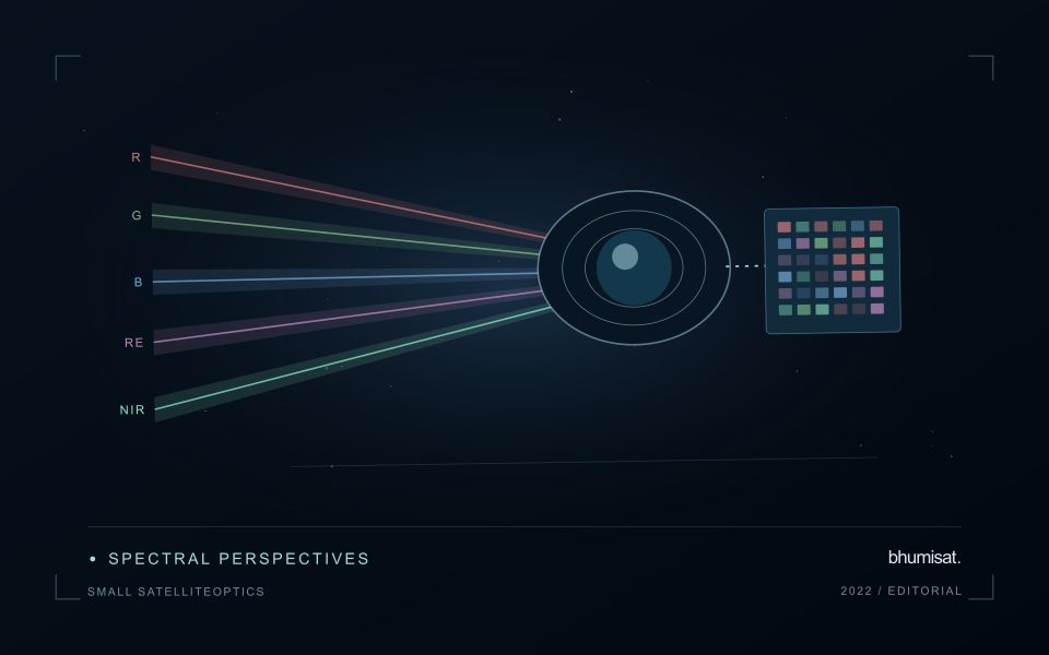
An optical Earth observation payload turns incoming radiance into sampled measurements. Its usefulness depends on more than the ground size represented by a pixel. The aperture, focal length, detector characteristics, spectral response and operating environment all influence the information that survives into the image. A mission should choose these features around a target measurement and its expected brightness, rather than treating pixel spacing as a complete performance specification.
Ground sampling distance describes the spacing of samples on the surface for a specified viewing geometry. Optical blur, detector response, motion and processing can reduce the detail that is actually resolved. The modulation transfer function expresses how contrast is retained across spatial frequencies and helps connect component performance with final image sharpness. Smaller pixels alone cannot recover detail removed by the optical system or excessive image motion.
Balance signal, packaging and calibration
A larger entrance aperture can collect more light, but it also creates demands on mass, volume, alignment and thermal control. Narrow spectral bands collect less energy than broader bands under otherwise comparable conditions. Longer integration can improve signal collection until motion, saturation or other constraints become limiting. The resulting trade must be evaluated for dark targets as well as bright land, and for the expected range of illumination and atmospheric conditions.
Small spacecraft packaging makes mechanical and thermal interfaces particularly consequential. Focus and alignment can shift as temperatures change, while launch loads and contamination can affect performance. Stray light from outside the intended field can bias measurements even when an image appears visually acceptable. Baffles, suitable materials, cleanliness procedures and representative testing help control these effects. Detector defects, nonuniform response and electronic noise also require characterization.
Plan radiometric, geometric and spectral calibration with the payload design. Establish how ground tests connect to measurements after launch, and how changes in response will be monitored. The calibration record should describe uncertainties and conditions, rather than just providing a correction file. Evaluate the complete imaging chain using representative scenes and realistic motion assumptions. A credible specification states where performance is expected, how it will be measured and which tradeoffs were accepted. It should not turn a detector data sheet into an unsupported claim about an entire spacecraft.
Locate the uncertainty that matters to the decision
An uncertainty budget is a practical description of where a result could become unreliable. Begin with the observation chain: acquisition, calibration, geographic matching, reference measurements, feature calculation, modelling, and delivery. Identify the assumptions at each stage and ask which could materially change the interpretation. The purpose is not to assign a precise number to every limitation. It is to locate the sources that deserve attention for the intended decision.
Separate limitations that can be measured from those that currently require a qualitative description. Repeated measurements may help characterise variability, while comparisons with independent references can reveal systematic differences. Some uncertainties interact, so combining individual error estimates without examining their relationships can produce a misleading impression of precision. Keep the method of assessment visible and avoid treating an unexamined assumption as though it were a negligible contribution.
Use the budget to prioritise further work. The largest visible source of variation is not always the one whose reduction would most improve the decision. Consider which additional observation, test, or contextual record would change confidence in an actionable way. Revisit the budget when the application, observation source, or deployment conditions change. This turns uncertainty analysis into a guide for improving the workflow rather than a qualification added only after the result has been delivered.
Match coastal observations with changing conditions
Coastal observations can be influenced by conditions that change within a day as well as across seasons. The meaning of an image or reference measurement may depend on water level, currents, recent weather, and the state of the surrounding land. Begin by documenting the exact acquisition time and the contextual records relevant to the question. A comparison based only on calendar dates can conceal differences that are important to interpretation.
Define which conditions need to be comparable across observations. A shoreline analysis, an intertidal habitat study, and an investigation of water appearance can require different timing assumptions. Select reference locations and measurement procedures that address the specific application. Preserve information about observation depth, sampling position, and the duration represented by a reference measurement where those details affect the comparison.
Review apparent differences against the physical and observational context before assigning a cause. A change in visible extent or spectral response may reflect the state of the water and atmosphere as well as a change in the feature being studied. Where suitable contextual information is unavailable, qualify the comparison or use additional observations to test competing explanations. A dependable coastal workflow makes its timing assumptions explicit and preserves the information needed to reconsider them when further evidence becomes available.
Bring the evidence back to the decision
Useful uncertainty communication identifies the limitation, explains how it could affect the result, and connects it to a practical response. Some decisions can proceed with a qualified estimate; others require another observation or an independent check. Preserve uncertainty information through processing and delivery so that it is available at the point of use. This makes the analysis more accountable and gives the team a clearer basis for deciding which additional evidence would most improve the outcome.
Sources & further reading
Explore the bhumisat spacecraft concept and our vision towards 2030, or return to the journal.