A workflow that succeeds on a small study area may encounter different constraints when the number of observations, locations, or users increases. Scaling requires attention to processing capacity, data organisation, reference coverage, and the effort needed to review results. This perspective looks beyond whether a calculation can run on a larger dataset. It asks whether the complete service can preserve its meaning, quality, and delivery commitments as its scope expands. The objective is a design that identifies bottlenecks early and increases throughput without silently weakening the evidence available to users.
This working guide considers optical payload choices for small satellites across coconut production landscapes. The immediate decision is to identify areas needing plantation review. Useful reference evidence includes palm spacing, understory condition and farm-level observations. The case is an illustrative planning context, with assumptions to check against the actual sensor, landscape and project requirements.
Connect the optical design to the measurement
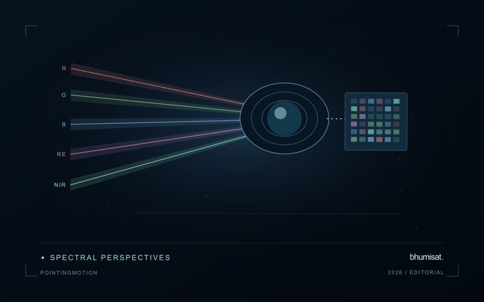
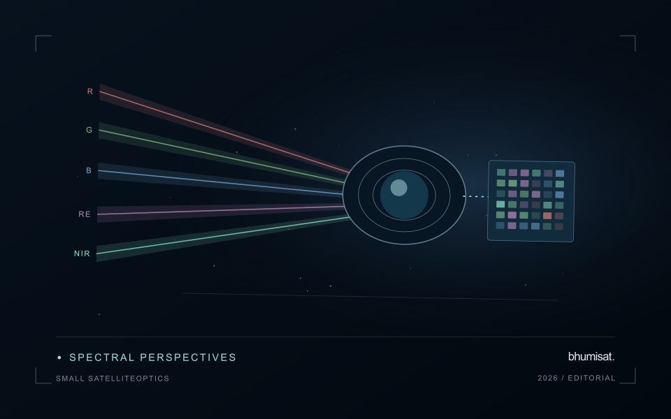
An optical Earth observation payload turns incoming radiance into sampled measurements. Its usefulness depends on more than the ground size represented by a pixel. The aperture, focal length, detector characteristics, spectral response and operating environment all influence the information that survives into the image. A mission should choose these features around a target measurement and its expected brightness, rather than treating pixel spacing as a complete performance specification.
Ground sampling distance describes the spacing of samples on the surface for a specified viewing geometry. Optical blur, detector response, motion and processing can reduce the detail that is actually resolved. The modulation transfer function expresses how contrast is retained across spatial frequencies and helps connect component performance with final image sharpness. Smaller pixels alone cannot recover detail removed by the optical system or excessive image motion.
Balance signal, packaging and calibration
A larger entrance aperture can collect more light, but it also creates demands on mass, volume, alignment and thermal control. Narrow spectral bands collect less energy than broader bands under otherwise comparable conditions. Longer integration can improve signal collection until motion, saturation or other constraints become limiting. The resulting trade must be evaluated for dark targets as well as bright land, and for the expected range of illumination and atmospheric conditions.
Small spacecraft packaging makes mechanical and thermal interfaces particularly consequential. Focus and alignment can shift as temperatures change, while launch loads and contamination can affect performance. Stray light from outside the intended field can bias measurements even when an image appears visually acceptable. Baffles, suitable materials, cleanliness procedures and representative testing help control these effects. Detector defects, nonuniform response and electronic noise also require characterization.
Plan radiometric, geometric and spectral calibration with the payload design. Establish how ground tests connect to measurements after launch, and how changes in response will be monitored. The calibration record should describe uncertainties and conditions, rather than just providing a correction file. Evaluate the complete imaging chain using representative scenes and realistic motion assumptions. A credible specification states where performance is expected, how it will be measured and which tradeoffs were accepted. It should not turn a detector data sheet into an unsupported claim about an entire spacecraft.
The setting: Coconut production landscapes
Coconut production landscapes can range from organised plantations to widely spaced palms embedded in farms, settlements and coastal vegetation. These settings create very different observation problems. A satellite pixel may combine palm crowns, soil, grass, roofs or water rather than represent coconut vegetation alone. Define whether the task is mapping a production landscape, documenting canopy change or studying a crop-specific variable before choosing an image product or interpretation method.
Field and management boundaries are important even where ownership units do not coincide with a continuous canopy. Record the extent of intercropping and other vegetation that may contribute to an observed change. In coastal settings, inspect shoreline adjacency, temporary flooding and atmospheric conditions alongside the imagery. A field-average vegetation response should be accompanied by the area and quality of the observations from which it was calculated.
Validation should describe palm arrangement, canopy continuity, understory and recent land-management events at known locations. Samples drawn only from dense or easily accessible stands may not represent the wider landscape. A model intended for crop condition or production needs reference measurements suited to that claim and evaluation beyond its development sites. For many users, a transparent inventory and a well-supported list of locations requiring review provide a practical foundation for later, more specialised analytical services.
Maintain the geographic units of analysis
Many observation services summarise measurements within a field, management block, catchment, forest unit, or other mapped boundary. The meaning of that summary depends on whether the boundary accurately represents the unit being discussed. Start with a clear source for the geometry and record its date, coordinate reference, and intended use. A boundary drawn for visual orientation may require additional checking before it becomes a measurement unit.
Inspect overlaps, gaps, narrow fragments, and features that may have changed since mapping. A geometrically valid polygon can still describe an outdated operational unit. Ask the responsible team how divisions, mergers, new infrastructure, and management changes are recorded. Where pixels or reference measurements cross a boundary, define how they are assigned or excluded so that results remain comparable between analysts and processing runs.
Version the boundaries alongside the observations. If a unit changes, preserve a relationship between the previous and revised geometry rather than replacing the history without explanation. Comparisons through time should identify whether they use a constant spatial unit or the operational units valid at each date. This makes it easier to distinguish a change in the measured surface from a change introduced by the geography used to summarise it.
Plan the evidence needed for calibration
Calibration connects an instrument's recorded response with a measurement that can be interpreted consistently. Begin by identifying which aspects of the response matter to the application: variation across channels, changes with operating conditions, geometric alignment, or differences between repeated observations. A calibration plan should state the quantities being assessed and the evidence needed to determine whether the response is sufficiently characterised for the intended use.
Design tests around controlled and documented conditions. Record the reference source, instrument configuration, exposure settings, temperature conditions, and processing applied to the measurements. Repeat suitable observations to investigate variability and distinguish a consistent response from a single favourable result. The reference itself has limitations, so preserve its characterisation and avoid assuming that every difference originates in the instrument under evaluation.
Connect calibration activities with the expected operating environment and processing chain. A correction that works under one test condition may require further evidence before being applied elsewhere. Define how calibration parameters are versioned, checked, and associated with the observations they support. Include a plan for recognising drift or other changes that could affect interpretation. The outcome should be an instrument response supported by traceable evidence, together with acceptance criteria that remain relevant to the application.
Bring the evidence back to the decision
Expansion should be guided by measured workload, visible quality conditions, and an understanding of which tasks require expert attention. Test the workflow under representative data volumes before treating a successful demonstration as evidence of operational capacity. Preserve a route for investigating individual observations even when most processing is automated. A scalable service keeps its results traceable and useful as it grows, with clear choices about where to automate, where to review, and where to invest in additional evidence.
Sources & further reading
Explore the bhumisat spacecraft concept and our vision towards 2030, or return to the journal.