A convincing image can still contain measurements that are unsuitable for a particular task. Quality control asks whether the inputs, transformations, and outputs meet the requirements of the intended application. This perspective follows evidence through the workflow, from acquisition metadata and reference observations to the final interpretation. It encourages teams to define acceptance conditions before seeing the result, rather than adjusting them to favour a preferred conclusion. The purpose is a repeatable way to distinguish usable observations, observations requiring qualification, and observations that should be excluded from a decision.
This working guide considers optical payload choices for small satellites around aquaculture pond clusters. The immediate decision is to prioritise pond-cluster monitoring visits. Useful reference evidence includes pond boundaries, operation status and timed water measurements. The case is an illustrative planning context, with assumptions to check against the actual sensor, landscape and project requirements.
The setting: Aquaculture pond clusters
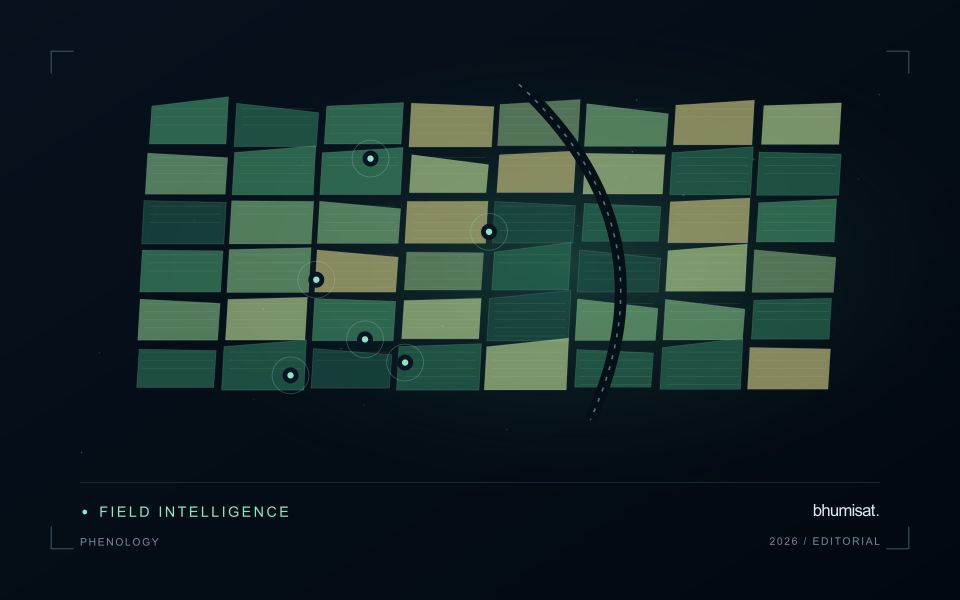
An aquaculture landscape contains ponds at different operating stages together with embankments, channels, roads and service areas. A satellite observation may support a pond inventory or a broader review of visible water patterns, but it should not be assumed to measure conditions within every individual production unit. Begin with boundaries and a record of pond status. Empty, recently filled and active ponds can have different appearances for ordinary operational reasons.
The size of a pond relative to the observation footprint determines how much embankment or neighbouring water contributes to a measurement. Review alignment and exclude unsuitable mixed areas where necessary. Surface reflections, cloud and atmospheric conditions can complicate optical comparison, while short-term management changes may occur between usable acquisitions. Retain observation dates and quality masks so that the image record does not imply continuous knowledge of rapidly changing pond conditions.
Validation should record the unit, collection time, operational context and the measurement method for any water variable being studied. A sample from one pond cannot automatically validate an adjacent pond or an entire cluster. A colour anomaly may help select a monitoring visit without establishing a particular biological condition or production outcome. More specific estimates require a demonstrated relationship with representative measurements, while inventory and inspection-priority products can be evaluated against the practical decisions they support.
Connect the optical design to the measurement
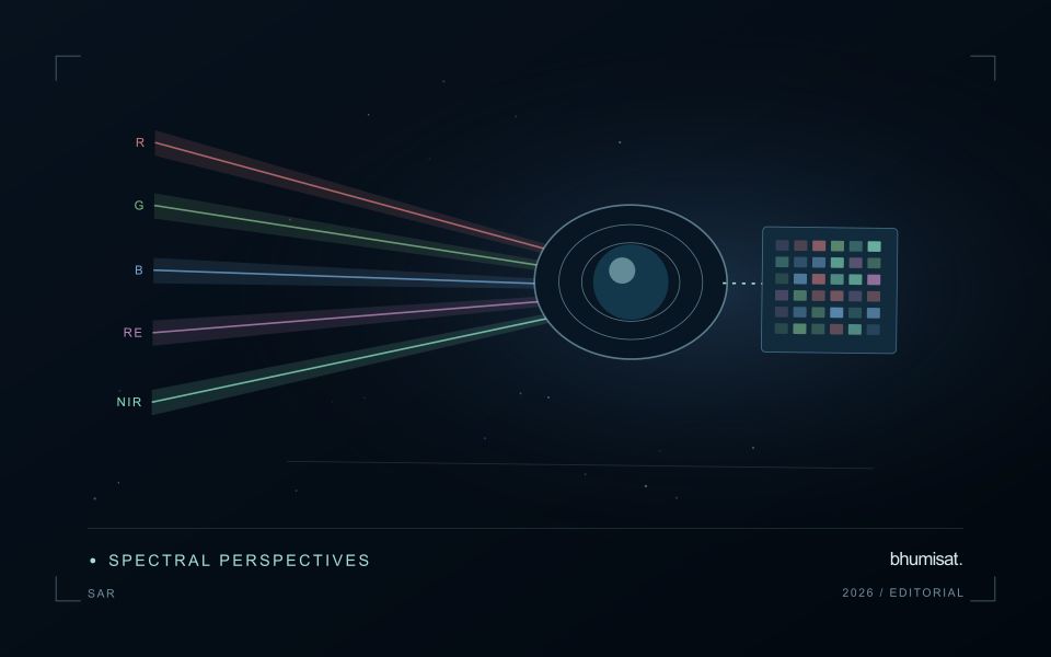
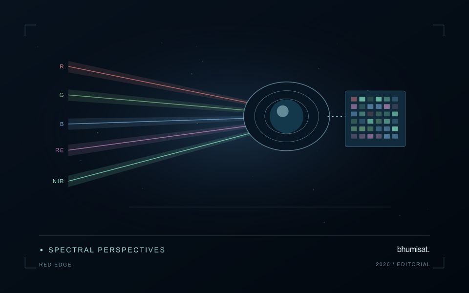
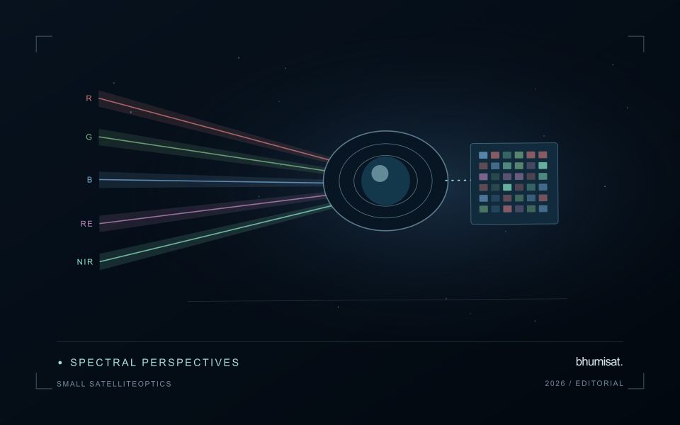
An optical Earth observation payload turns incoming radiance into sampled measurements. Its usefulness depends on more than the ground size represented by a pixel. The aperture, focal length, detector characteristics, spectral response and operating environment all influence the information that survives into the image. A mission should choose these features around a target measurement and its expected brightness, rather than treating pixel spacing as a complete performance specification.
Ground sampling distance describes the spacing of samples on the surface for a specified viewing geometry. Optical blur, detector response, motion and processing can reduce the detail that is actually resolved. The modulation transfer function expresses how contrast is retained across spatial frequencies and helps connect component performance with final image sharpness. Smaller pixels alone cannot recover detail removed by the optical system or excessive image motion.
Balance signal, packaging and calibration
A larger entrance aperture can collect more light, but it also creates demands on mass, volume, alignment and thermal control. Narrow spectral bands collect less energy than broader bands under otherwise comparable conditions. Longer integration can improve signal collection until motion, saturation or other constraints become limiting. The resulting trade must be evaluated for dark targets as well as bright land, and for the expected range of illumination and atmospheric conditions.
Small spacecraft packaging makes mechanical and thermal interfaces particularly consequential. Focus and alignment can shift as temperatures change, while launch loads and contamination can affect performance. Stray light from outside the intended field can bias measurements even when an image appears visually acceptable. Baffles, suitable materials, cleanliness procedures and representative testing help control these effects. Detector defects, nonuniform response and electronic noise also require characterization.
Plan radiometric, geometric and spectral calibration with the payload design. Establish how ground tests connect to measurements after launch, and how changes in response will be monitored. The calibration record should describe uncertainties and conditions, rather than just providing a correction file. Evaluate the complete imaging chain using representative scenes and realistic motion assumptions. A credible specification states where performance is expected, how it will be measured and which tradeoffs were accepted. It should not turn a detector data sheet into an unsupported claim about an entire spacecraft.
Check spatial alignment before comparison
A comparison between images, channels, maps, or field measurements assumes that the observations refer to the same locations at a suitable level of precision. Small alignment errors can become especially important near boundaries or narrow features. Before interpreting differences, inspect whether identifiable, stable features agree between the sources. A common coordinate reference is necessary for many workflows, but it does not by itself demonstrate accurate alignment.
Use control features that are appropriate for the observation scale and remain stable across the comparison period. Evaluate alignment in more than one part of the area, because a single location cannot reveal spatially varying distortion. Record the method used to estimate any correction and retain independent features for checking the corrected result. Where surfaces have genuinely changed, avoid using those changes as evidence of an alignment error.
Propagate the implications of remaining misalignment into the analysis. A workflow may exclude boundary pixels, summarise at a broader scale, or qualify interpretations for small features. The choice should follow the application rather than a preference for visually smooth output. Preserve both the original and corrected geographic references, and document resampling decisions so that future users can understand how measurements were moved onto a common spatial framework.
Represent gaps without inventing observations
A monitoring sequence often contains periods without a usable observation. The reason may be cloud, shadow, missing coverage, a failed transfer, or a quality condition that excludes the data. Begin by representing these states explicitly. A missing observation is different from a low measurement, an unchanged surface, or a confirmed absence of the feature being studied. The distinction should survive both the analysis and the presentation of the result.
Define when a temporal gap is acceptable for the intended decision. A workflow may continue using the latest qualified observation, request another source, or suspend an alert until sufficient evidence is available. Whichever response is selected, show the age of the supporting observation. If interpolation is used for a suitable analytical purpose, preserve the distinction between an estimated value and a directly observed measurement, together with the assumptions needed to interpret it.
Review how gaps affect the coverage of the final evaluation. Locations with frequent missing data may differ systematically from those with regular observations. A performance estimate based only on clear, complete records can therefore describe a narrower population than the service is expected to support. Report usable coverage alongside analytical results and use recurring gaps to guide acquisition planning, reference collection, and the selection of complementary observation methods.
Bring the evidence back to the decision
Quality control is most useful when its results travel with the information being delivered. Preserve the reasons for accepting or rejecting an observation, and expose limitations that could change the user's interpretation. Review recurring failures as clues about the design of the workflow. A clear quality record supports consistent comparisons between operators and processing versions, while helping the team decide whether a problem originates in acquisition, preparation, interpretation, or the underlying observation requirements.
Sources & further reading
Explore the bhumisat spacecraft concept and our vision towards 2030, or return to the journal.