A useful observation programme begins with a decision that somebody can act on. Before selecting imagery or instruments, define the area of interest, the people responsible for inspecting it, and the time available for a response. This planning perspective connects remote measurements with the practical questions that shape a survey or monitoring service. The aim is to identify which observations would change a decision, how supporting evidence would be collected, and what should happen when information is incomplete. A clear plan makes later technical choices easier to assess against an operational purpose.
This working guide considers synthetic aperture radar for land monitoring across estuarine mixing zones. The immediate decision is to plan sampling across estuarine gradients. Useful reference evidence includes tidal stage, sample timing and water-variable measurements. The case is an illustrative planning context, with assumptions to check against the actual sensor, landscape and project requirements.
Radar measures a different interaction with the landscape
Synthetic aperture radar is an active observing technique: the instrument transmits microwave energy and measures the returned signal. Its image therefore represents a different interaction with the landscape from reflected visible or near-infrared sunlight. Radar can provide observations in conditions that limit optical imagery, but its response still depends on the instrument and scene. Backscatter should not be read as a universal moisture or vegetation score. Surface structure, water, roughness, geometry and the arrangement of scattering elements can contribute to the measured return.
Wavelength and polarisation influence which interactions are emphasised. The same agricultural field can change its radar response after rainfall, tillage, crop development or harvest, and several of those processes may occur together. The viewing direction and incidence angle also matter. A time series assembled without controlling these factors can contain differences that look like an environmental trend. Retain orbit, geometry, polarisation and processing metadata, and choose comparisons that are appropriate for the physical interpretation the application is intended to support.
Compare like with like before drawing conclusions
Radar images commonly contain speckle, a granular appearance associated with coherent measurement. Filtering or aggregation can make patterns easier to interpret, but it also changes spatial detail and statistical behaviour. Select processing around the reporting scale and evaluate its effects near boundaries. Terrain can create additional geometric challenges, including compressed or hidden areas in the radar view. A map should identify where the observation is difficult to interpret rather than filling every location with an equally confident result.
Complementary evidence helps distinguish plausible explanations for a radar change. Combine suitable optical observations, rainfall or management records and field measurements when they address the actual question. Validate a proposed model on independent locations and conditions, including cases where the expected relationship fails. A dark water surface in one setting does not establish a universal flood rule, because rough water, vegetation and built structures can produce different responses. Radar becomes valuable when its particular measurement physics is incorporated into a carefully defined monitoring workflow, with geometry and uncertainty remaining visible to the analyst and user.
The setting: Estuarine mixing zones
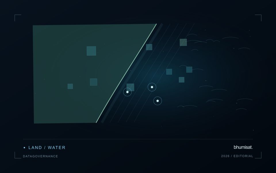
An estuary connects river inflow, coastal water, tidal conditions and complex shorelines. The resulting image pattern may change even when a monitoring team has not altered its methods. A useful design begins with a specific question, such as mapping visible water or investigating a persistent spectral gradient. It should not assume that one relationship describes every part of the estuary or that a single acquisition represents conditions throughout a tidal cycle.
Comparison units should account for channels, shallow margins and locations where land and water are mixed within an observation. Review cloud and atmospheric quality, surface reflection and geometric alignment before interpreting a difference between dates. Tidal and inflow context can help explain the setting but does not replace measurements of the target variable. Preserve the acquisition times and valid areas so that a mapped feature can be evaluated against the conditions under which it was observed.
A validation plan should represent different water types and spatial positions across the mixing zone. Collect the timing and location of samples consistently, and consider whether conditions changed between sampling and acquisition. A spectral boundary may help organise an investigation without proving a particular source or ecological consequence. More specific interpretations require evidence designed for those claims, while an auditable record of observed patterns and sampling priorities can already improve the structure of a monitoring programme.
Plan the evidence needed for calibration
Calibration connects an instrument's recorded response with a measurement that can be interpreted consistently. Begin by identifying which aspects of the response matter to the application: variation across channels, changes with operating conditions, geometric alignment, or differences between repeated observations. A calibration plan should state the quantities being assessed and the evidence needed to determine whether the response is sufficiently characterised for the intended use.
Design tests around controlled and documented conditions. Record the reference source, instrument configuration, exposure settings, temperature conditions, and processing applied to the measurements. Repeat suitable observations to investigate variability and distinguish a consistent response from a single favourable result. The reference itself has limitations, so preserve its characterisation and avoid assuming that every difference originates in the instrument under evaluation.
Connect calibration activities with the expected operating environment and processing chain. A correction that works under one test condition may require further evidence before being applied elsewhere. Define how calibration parameters are versioned, checked, and associated with the observations they support. Include a plan for recognising drift or other changes that could affect interpretation. The outcome should be an instrument response supported by traceable evidence, together with acceptance criteria that remain relevant to the application.
Maintain the geographic units of analysis
Many observation services summarise measurements within a field, management block, catchment, forest unit, or other mapped boundary. The meaning of that summary depends on whether the boundary accurately represents the unit being discussed. Start with a clear source for the geometry and record its date, coordinate reference, and intended use. A boundary drawn for visual orientation may require additional checking before it becomes a measurement unit.
Inspect overlaps, gaps, narrow fragments, and features that may have changed since mapping. A geometrically valid polygon can still describe an outdated operational unit. Ask the responsible team how divisions, mergers, new infrastructure, and management changes are recorded. Where pixels or reference measurements cross a boundary, define how they are assigned or excluded so that results remain comparable between analysts and processing runs.
Version the boundaries alongside the observations. If a unit changes, preserve a relationship between the previous and revised geometry rather than replacing the history without explanation. Comparisons through time should identify whether they use a constant spatial unit or the operational units valid at each date. This makes it easier to distinguish a change in the measured surface from a change introduced by the geography used to summarise it.
Bring the evidence back to the decision
The practical outcome should be a short observation plan that another team can follow. It should name the decision, the required evidence, the responsible roles, and the conditions that trigger a field visit or further analysis. Keep the plan small enough to test, then revise it using the results of real inspections. A useful monitoring workflow improves because its assumptions are examined systematically, and its observations remain connected to decisions throughout the process.
Sources & further reading
Explore the bhumisat spacecraft concept and our vision towards 2030, or return to the journal.