Comparisons through time are valuable only when the observations are sufficiently comparable for the question being asked. A difference between dates can reflect real change, a normal stage in a seasonal cycle, or a difference in how the surface was observed. This perspective examines the reference period, the timing of acquisitions, and the contextual records needed to interpret a sequence. It encourages the use of appropriate baselines rather than treating every previous observation as an equivalent benchmark. The objective is to identify changes that remain meaningful after normal variation and measurement conditions are considered.
This working guide considers red edge sensing for vegetation studies in potato growing fields. The immediate decision is to focus scouting within potato fields. Useful reference evidence includes emergence records, canopy stage and representative plot observations. The case is an illustrative planning context, with assumptions to check against the actual sensor, landscape and project requirements.
Observe a transition, not a universal plant score
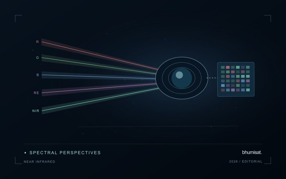
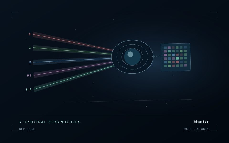
The Red Edge is a transition region in the spectral response of vegetation between visible red absorption and near-infrared reflectance. Measuring this region can add useful information to a vegetation study because different channels sample different parts of the transition. The phrase Red Edge is therefore a broad description rather than a complete instrument specification. A study needs the channel response, its bandwidth and its relationship to the other measurements used in the analysis. Those details influence what comparisons can be made reliably.
Leaf properties and the arrangement of leaves within a canopy both affect the signal reaching a satellite. The observed field also contains shadows, branches, soil and sometimes water or understory vegetation. Consequently, a relationship established with a leaf instrument cannot simply be assumed to hold at satellite-pixel scale. Scaling the interpretation requires observations that connect these levels. This distinction becomes especially important when the intended application concerns a specific biochemical parameter, because the image records a combined landscape response rather than an isolated leaf measurement.
Design the comparison around the instrument
Start an application study by identifying the information that an added Red Edge channel is expected to contribute. Compare that expectation with available data from established instruments and with a baseline method using fewer bands. Check whether any apparent improvement persists in independent fields and seasons. Use the same evaluation protocol for both methods. An instrument design decision should consider the improvement alongside calibration, alignment, signal quality and processing demands. More channels introduce more measurement opportunities and more relationships that must be understood.
For an ongoing service, retain enough metadata to trace every result to its source bands. A change in sensor, processing version or band selection can create a discontinuity in an otherwise plausible time series. Validate the transition rather than hiding it within a long historical chart. Clear documentation allows a user to distinguish a change in vegetation from a change in the observation system. Red Edge sensing becomes valuable when its additional spectral information can be linked to a defined application through repeatable measurements and independent evidence.
The setting: Potato growing fields
Potato monitoring begins with the distinction between the canopy visible from above and the crop component ultimately harvested below ground. Establishment timing, variety, row structure and management can create different canopy patterns across fields. An image service should specify whether it is supporting crop-stage assessment, identifying areas for inspection or estimating a defined production variable. These objectives require different reference measurements and should not be combined into one unqualified vegetation score.
Maintain a field timeline that includes planting, emergence and the operations that can affect canopy appearance. Early observations may contain a large soil contribution, while later observations may show a more continuous canopy. Cloud and shadow contamination, field edges and neighbouring land cover can alter summaries at either stage. Compare observations using suitable quality rules and retain the acquisition dates so that a recent-looking map does not conceal an old measurement.
A field team should collect consistent crop-stage and canopy observations across both flagged and typical areas. Record management context and sampling support rather than relying on an isolated photograph. A vegetation change cannot establish the presence of a specific disease, and a canopy index is not a direct measurement of tuber yield. Evaluate any production model with appropriate harvest data and independent assessment, while keeping the simpler inspection-priority product transparent about what it actually observes.
Maintain the geographic units of analysis
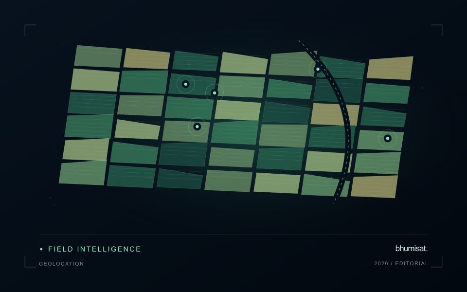
Many observation services summarise measurements within a field, management block, catchment, forest unit, or other mapped boundary. The meaning of that summary depends on whether the boundary accurately represents the unit being discussed. Start with a clear source for the geometry and record its date, coordinate reference, and intended use. A boundary drawn for visual orientation may require additional checking before it becomes a measurement unit.
Inspect overlaps, gaps, narrow fragments, and features that may have changed since mapping. A geometrically valid polygon can still describe an outdated operational unit. Ask the responsible team how divisions, mergers, new infrastructure, and management changes are recorded. Where pixels or reference measurements cross a boundary, define how they are assigned or excluded so that results remain comparable between analysts and processing runs.
Version the boundaries alongside the observations. If a unit changes, preserve a relationship between the previous and revised geometry rather than replacing the history without explanation. Comparisons through time should identify whether they use a constant spatial unit or the operational units valid at each date. This makes it easier to distinguish a change in the measured surface from a change introduced by the geography used to summarise it.
Plan the evidence needed for calibration
Calibration connects an instrument's recorded response with a measurement that can be interpreted consistently. Begin by identifying which aspects of the response matter to the application: variation across channels, changes with operating conditions, geometric alignment, or differences between repeated observations. A calibration plan should state the quantities being assessed and the evidence needed to determine whether the response is sufficiently characterised for the intended use.
Design tests around controlled and documented conditions. Record the reference source, instrument configuration, exposure settings, temperature conditions, and processing applied to the measurements. Repeat suitable observations to investigate variability and distinguish a consistent response from a single favourable result. The reference itself has limitations, so preserve its characterisation and avoid assuming that every difference originates in the instrument under evaluation.
Connect calibration activities with the expected operating environment and processing chain. A correction that works under one test condition may require further evidence before being applied elsewhere. Define how calibration parameters are versioned, checked, and associated with the observations they support. Include a plan for recognising drift or other changes that could affect interpretation. The outcome should be an instrument response supported by traceable evidence, together with acceptance criteria that remain relevant to the application.
Bring the evidence back to the decision
A useful comparison preserves the dates, quality conditions, and contextual assumptions behind its baseline. Review unusual results against the actual observation sequence rather than relying entirely on a summary statistic. Where seasonal timing is important, describe how comparable stages were identified. The resulting analysis should help users distinguish an informative change from an expected cycle or an observation artefact, while making gaps and remaining uncertainty visible enough to guide further investigation.
Sources & further reading
Explore the bhumisat spacecraft concept and our vision towards 2030, or return to the journal.