Every observation and interpretation contains uncertainty, but the sources and consequences of that uncertainty differ between applications. Some arise from acquisition conditions, others from reference measurements, processing choices, or the transfer of a model to a new setting. This perspective examines how those sources affect the decision a user is considering. It encourages teams to describe uncertainty in a form that can influence action, rather than adding a generic qualification at the end of a report. The objective is to support proportionate decisions while keeping the limits of the available evidence understandable.
This working guide considers red edge sensing for vegetation studies along mangrove forest margins. The immediate decision is to review changing mangrove cover. Useful reference evidence includes tidal context, canopy boundaries and representative field plots. The case is an illustrative planning context, with assumptions to check against the actual sensor, landscape and project requirements.
The setting: Mangrove forest margins
Mangrove monitoring takes place at a changing boundary between land and water. The observed surface depends on canopy structure, tidal conditions, exposed sediment and the arrangement of channels. A narrow fringe may contain a high proportion of mixed observations even when the surrounding image appears detailed. Begin by defining whether the task is mapping canopy extent, detecting disturbance or studying a forest attribute, and establish the spatial unit that the data can represent defensibly.
Comparisons between dates should account for water and sediment conditions as well as cloud, haze and shadow. A change near the canopy edge may reflect different water exposure or geometric alignment rather than a new loss of trees. Retain the acquisition dates and relevant tidal context where available. Mapping rules should distinguish canopy, water and other surfaces consistently, while acknowledging locations where their contributions cannot be separated reliably at the chosen resolution.
Field observations should describe canopy boundaries, vegetation structure and the setting of sampled plots or inspection points. Record whether a visit represents an edge, a channel margin or the forest interior. A mapped vegetation response alone cannot establish carbon stock, habitat quality or the cause of a disturbance. Those interpretations need suitable evidence. A practical initial product provides a traceable cover-change assessment and a prioritised set of locations where field review would resolve important uncertainty.
Observe a transition, not a universal plant score
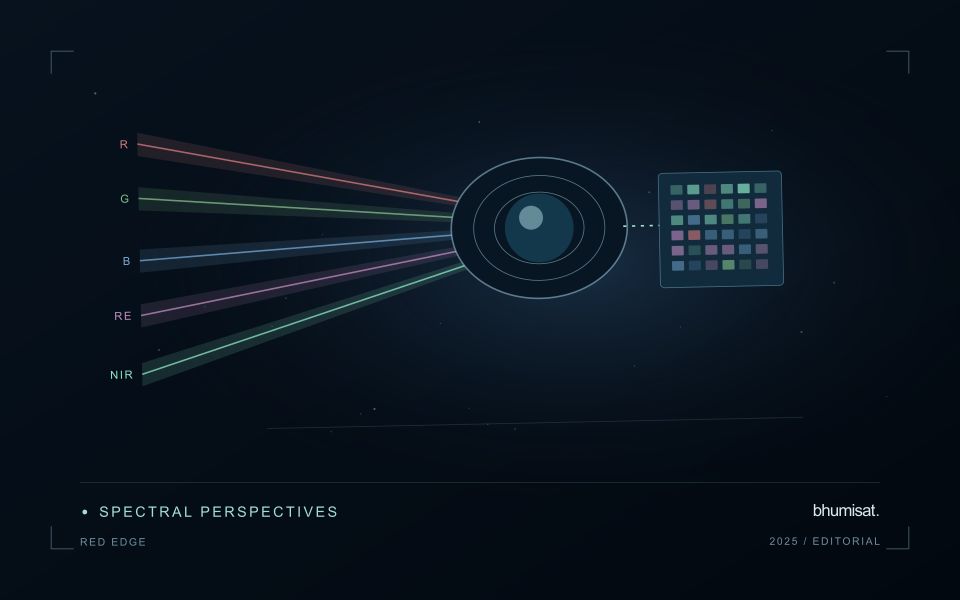
The Red Edge is a transition region in the spectral response of vegetation between visible red absorption and near-infrared reflectance. Measuring this region can add useful information to a vegetation study because different channels sample different parts of the transition. The phrase Red Edge is therefore a broad description rather than a complete instrument specification. A study needs the channel response, its bandwidth and its relationship to the other measurements used in the analysis. Those details influence what comparisons can be made reliably.
Leaf properties and the arrangement of leaves within a canopy both affect the signal reaching a satellite. The observed field also contains shadows, branches, soil and sometimes water or understory vegetation. Consequently, a relationship established with a leaf instrument cannot simply be assumed to hold at satellite-pixel scale. Scaling the interpretation requires observations that connect these levels. This distinction becomes especially important when the intended application concerns a specific biochemical parameter, because the image records a combined landscape response rather than an isolated leaf measurement.
Design the comparison around the instrument
Start an application study by identifying the information that an added Red Edge channel is expected to contribute. Compare that expectation with available data from established instruments and with a baseline method using fewer bands. Check whether any apparent improvement persists in independent fields and seasons. Use the same evaluation protocol for both methods. An instrument design decision should consider the improvement alongside calibration, alignment, signal quality and processing demands. More channels introduce more measurement opportunities and more relationships that must be understood.
For an ongoing service, retain enough metadata to trace every result to its source bands. A change in sensor, processing version or band selection can create a discontinuity in an otherwise plausible time series. Validate the transition rather than hiding it within a long historical chart. Clear documentation allows a user to distinguish a change in vegetation from a change in the observation system. Red Edge sensing becomes valuable when its additional spectral information can be linked to a defined application through repeatable measurements and independent evidence.
Check spatial alignment before comparison
A comparison between images, channels, maps, or field measurements assumes that the observations refer to the same locations at a suitable level of precision. Small alignment errors can become especially important near boundaries or narrow features. Before interpreting differences, inspect whether identifiable, stable features agree between the sources. A common coordinate reference is necessary for many workflows, but it does not by itself demonstrate accurate alignment.
Use control features that are appropriate for the observation scale and remain stable across the comparison period. Evaluate alignment in more than one part of the area, because a single location cannot reveal spatially varying distortion. Record the method used to estimate any correction and retain independent features for checking the corrected result. Where surfaces have genuinely changed, avoid using those changes as evidence of an alignment error.
Propagate the implications of remaining misalignment into the analysis. A workflow may exclude boundary pixels, summarise at a broader scale, or qualify interpretations for small features. The choice should follow the application rather than a preference for visually smooth output. Preserve both the original and corrected geographic references, and document resampling decisions so that future users can understand how measurements were moved onto a common spatial framework.
Locate the uncertainty that matters to the decision
An uncertainty budget is a practical description of where a result could become unreliable. Begin with the observation chain: acquisition, calibration, geographic matching, reference measurements, feature calculation, modelling, and delivery. Identify the assumptions at each stage and ask which could materially change the interpretation. The purpose is not to assign a precise number to every limitation. It is to locate the sources that deserve attention for the intended decision.
Separate limitations that can be measured from those that currently require a qualitative description. Repeated measurements may help characterise variability, while comparisons with independent references can reveal systematic differences. Some uncertainties interact, so combining individual error estimates without examining their relationships can produce a misleading impression of precision. Keep the method of assessment visible and avoid treating an unexamined assumption as though it were a negligible contribution.
Use the budget to prioritise further work. The largest visible source of variation is not always the one whose reduction would most improve the decision. Consider which additional observation, test, or contextual record would change confidence in an actionable way. Revisit the budget when the application, observation source, or deployment conditions change. This turns uncertainty analysis into a guide for improving the workflow rather than a qualification added only after the result has been delivered.
Bring the evidence back to the decision
Useful uncertainty communication identifies the limitation, explains how it could affect the result, and connects it to a practical response. Some decisions can proceed with a qualified estimate; others require another observation or an independent check. Preserve uncertainty information through processing and delivery so that it is available at the point of use. This makes the analysis more accountable and gives the team a clearer basis for deciding which additional evidence would most improve the outcome.
Sources & further reading
Explore the bhumisat spacecraft concept and our vision towards 2030, or return to the journal.