Every observation and interpretation contains uncertainty, but the sources and consequences of that uncertainty differ between applications. Some arise from acquisition conditions, others from reference measurements, processing choices, or the transfer of a model to a new setting. This perspective examines how those sources affect the decision a user is considering. It encourages teams to describe uncertainty in a form that can influence action, rather than adding a generic qualification at the end of a report. The objective is to support proportionate decisions while keeping the limits of the available evidence understandable.
This working guide considers red edge sensing for vegetation studies across estuarine mixing zones. The immediate decision is to plan sampling across estuarine gradients. Useful reference evidence includes tidal stage, sample timing and water-variable measurements. The case is an illustrative planning context, with assumptions to check against the actual sensor, landscape and project requirements.
Observe a transition, not a universal plant score
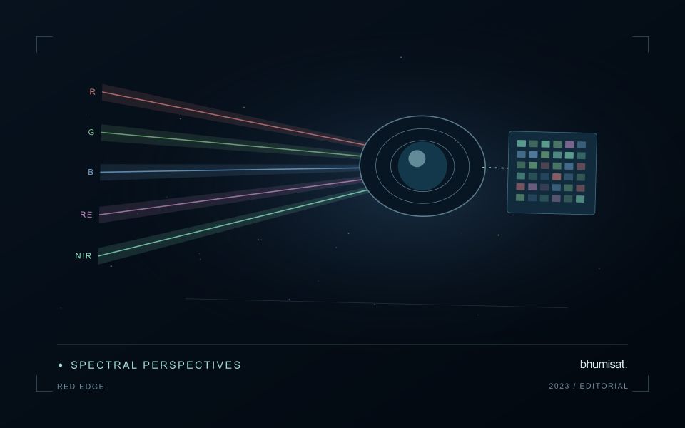
The Red Edge is a transition region in the spectral response of vegetation between visible red absorption and near-infrared reflectance. Measuring this region can add useful information to a vegetation study because different channels sample different parts of the transition. The phrase Red Edge is therefore a broad description rather than a complete instrument specification. A study needs the channel response, its bandwidth and its relationship to the other measurements used in the analysis. Those details influence what comparisons can be made reliably.
Leaf properties and the arrangement of leaves within a canopy both affect the signal reaching a satellite. The observed field also contains shadows, branches, soil and sometimes water or understory vegetation. Consequently, a relationship established with a leaf instrument cannot simply be assumed to hold at satellite-pixel scale. Scaling the interpretation requires observations that connect these levels. This distinction becomes especially important when the intended application concerns a specific biochemical parameter, because the image records a combined landscape response rather than an isolated leaf measurement.
Design the comparison around the instrument
Start an application study by identifying the information that an added Red Edge channel is expected to contribute. Compare that expectation with available data from established instruments and with a baseline method using fewer bands. Check whether any apparent improvement persists in independent fields and seasons. Use the same evaluation protocol for both methods. An instrument design decision should consider the improvement alongside calibration, alignment, signal quality and processing demands. More channels introduce more measurement opportunities and more relationships that must be understood.
For an ongoing service, retain enough metadata to trace every result to its source bands. A change in sensor, processing version or band selection can create a discontinuity in an otherwise plausible time series. Validate the transition rather than hiding it within a long historical chart. Clear documentation allows a user to distinguish a change in vegetation from a change in the observation system. Red Edge sensing becomes valuable when its additional spectral information can be linked to a defined application through repeatable measurements and independent evidence.
The setting: Estuarine mixing zones
An estuary connects river inflow, coastal water, tidal conditions and complex shorelines. The resulting image pattern may change even when a monitoring team has not altered its methods. A useful design begins with a specific question, such as mapping visible water or investigating a persistent spectral gradient. It should not assume that one relationship describes every part of the estuary or that a single acquisition represents conditions throughout a tidal cycle.
Comparison units should account for channels, shallow margins and locations where land and water are mixed within an observation. Review cloud and atmospheric quality, surface reflection and geometric alignment before interpreting a difference between dates. Tidal and inflow context can help explain the setting but does not replace measurements of the target variable. Preserve the acquisition times and valid areas so that a mapped feature can be evaluated against the conditions under which it was observed.
A validation plan should represent different water types and spatial positions across the mixing zone. Collect the timing and location of samples consistently, and consider whether conditions changed between sampling and acquisition. A spectral boundary may help organise an investigation without proving a particular source or ecological consequence. More specific interpretations require evidence designed for those claims, while an auditable record of observed patterns and sampling priorities can already improve the structure of a monitoring programme.
Use observation labels with consistent meanings
A reference label should describe an observation that another person could recognise or reproduce. Broad terms such as good, damaged, or unusual can conceal substantial differences between collection teams. Begin by defining the feature or condition being recorded, the observation unit, and the evidence needed to assign a label. Where possible, distinguish a direct measurement from an interpretation made by the observer.
Provide a short collection guide with examples, boundary cases, and a way to record uncertainty. Train observers using shared cases before relying on independently collected labels. If two observers disagree, preserve the disagreement long enough to understand its cause. It may reveal an unclear definition, a genuinely ambiguous condition, a difference in observation scale, or a problem in matching the reference record to the remote measurement.
Retain the context that makes the label interpretable. Location, time, collection method, observer role, and relevant surface conditions can be essential for later review. Changes to the label scheme should be documented and related to earlier versions where a defensible correspondence exists. Consistent labels do not eliminate uncertainty, but they make it possible to investigate disagreement, evaluate analytical methods, and identify where better definitions or additional measurements would improve the evidence.
Maintain the geographic units of analysis
Many observation services summarise measurements within a field, management block, catchment, forest unit, or other mapped boundary. The meaning of that summary depends on whether the boundary accurately represents the unit being discussed. Start with a clear source for the geometry and record its date, coordinate reference, and intended use. A boundary drawn for visual orientation may require additional checking before it becomes a measurement unit.
Inspect overlaps, gaps, narrow fragments, and features that may have changed since mapping. A geometrically valid polygon can still describe an outdated operational unit. Ask the responsible team how divisions, mergers, new infrastructure, and management changes are recorded. Where pixels or reference measurements cross a boundary, define how they are assigned or excluded so that results remain comparable between analysts and processing runs.
Version the boundaries alongside the observations. If a unit changes, preserve a relationship between the previous and revised geometry rather than replacing the history without explanation. Comparisons through time should identify whether they use a constant spatial unit or the operational units valid at each date. This makes it easier to distinguish a change in the measured surface from a change introduced by the geography used to summarise it.
Bring the evidence back to the decision
Useful uncertainty communication identifies the limitation, explains how it could affect the result, and connects it to a practical response. Some decisions can proceed with a qualified estimate; others require another observation or an independent check. Preserve uncertainty information through processing and delivery so that it is available at the point of use. This makes the analysis more accountable and gives the team a clearer basis for deciding which additional evidence would most improve the outcome.
Sources & further reading
Explore the bhumisat spacecraft concept and our vision towards 2030, or return to the journal.