A workflow that succeeds on a small study area may encounter different constraints when the number of observations, locations, or users increases. Scaling requires attention to processing capacity, data organisation, reference coverage, and the effort needed to review results. This perspective looks beyond whether a calculation can run on a larger dataset. It asks whether the complete service can preserve its meaning, quality, and delivery commitments as its scope expands. The objective is a design that identifies bottlenecks early and increases throughput without silently weakening the evidence available to users.
This working guide considers red edge sensing for vegetation studies across estuarine mixing zones. The immediate decision is to plan sampling across estuarine gradients. Useful reference evidence includes tidal stage, sample timing and water-variable measurements. The case is an illustrative planning context, with assumptions to check against the actual sensor, landscape and project requirements.
Observe a transition, not a universal plant score
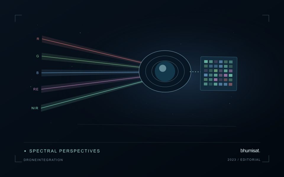
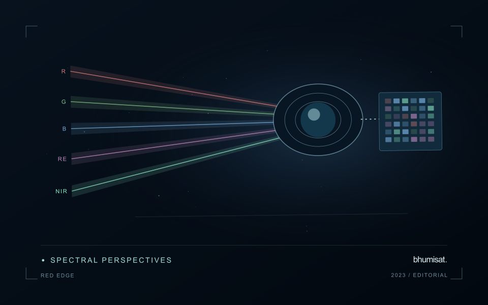
The Red Edge is a transition region in the spectral response of vegetation between visible red absorption and near-infrared reflectance. Measuring this region can add useful information to a vegetation study because different channels sample different parts of the transition. The phrase Red Edge is therefore a broad description rather than a complete instrument specification. A study needs the channel response, its bandwidth and its relationship to the other measurements used in the analysis. Those details influence what comparisons can be made reliably.
Leaf properties and the arrangement of leaves within a canopy both affect the signal reaching a satellite. The observed field also contains shadows, branches, soil and sometimes water or understory vegetation. Consequently, a relationship established with a leaf instrument cannot simply be assumed to hold at satellite-pixel scale. Scaling the interpretation requires observations that connect these levels. This distinction becomes especially important when the intended application concerns a specific biochemical parameter, because the image records a combined landscape response rather than an isolated leaf measurement.
Design the comparison around the instrument
Start an application study by identifying the information that an added Red Edge channel is expected to contribute. Compare that expectation with available data from established instruments and with a baseline method using fewer bands. Check whether any apparent improvement persists in independent fields and seasons. Use the same evaluation protocol for both methods. An instrument design decision should consider the improvement alongside calibration, alignment, signal quality and processing demands. More channels introduce more measurement opportunities and more relationships that must be understood.
For an ongoing service, retain enough metadata to trace every result to its source bands. A change in sensor, processing version or band selection can create a discontinuity in an otherwise plausible time series. Validate the transition rather than hiding it within a long historical chart. Clear documentation allows a user to distinguish a change in vegetation from a change in the observation system. Red Edge sensing becomes valuable when its additional spectral information can be linked to a defined application through repeatable measurements and independent evidence.
The setting: Estuarine mixing zones
An estuary connects river inflow, coastal water, tidal conditions and complex shorelines. The resulting image pattern may change even when a monitoring team has not altered its methods. A useful design begins with a specific question, such as mapping visible water or investigating a persistent spectral gradient. It should not assume that one relationship describes every part of the estuary or that a single acquisition represents conditions throughout a tidal cycle.
Comparison units should account for channels, shallow margins and locations where land and water are mixed within an observation. Review cloud and atmospheric quality, surface reflection and geometric alignment before interpreting a difference between dates. Tidal and inflow context can help explain the setting but does not replace measurements of the target variable. Preserve the acquisition times and valid areas so that a mapped feature can be evaluated against the conditions under which it was observed.
A validation plan should represent different water types and spatial positions across the mixing zone. Collect the timing and location of samples consistently, and consider whether conditions changed between sampling and acquisition. A spectral boundary may help organise an investigation without proving a particular source or ecological consequence. More specific interpretations require evidence designed for those claims, while an auditable record of observed patterns and sampling priorities can already improve the structure of a monitoring programme.
Check spatial alignment before comparison
A comparison between images, channels, maps, or field measurements assumes that the observations refer to the same locations at a suitable level of precision. Small alignment errors can become especially important near boundaries or narrow features. Before interpreting differences, inspect whether identifiable, stable features agree between the sources. A common coordinate reference is necessary for many workflows, but it does not by itself demonstrate accurate alignment.
Use control features that are appropriate for the observation scale and remain stable across the comparison period. Evaluate alignment in more than one part of the area, because a single location cannot reveal spatially varying distortion. Record the method used to estimate any correction and retain independent features for checking the corrected result. Where surfaces have genuinely changed, avoid using those changes as evidence of an alignment error.
Propagate the implications of remaining misalignment into the analysis. A workflow may exclude boundary pixels, summarise at a broader scale, or qualify interpretations for small features. The choice should follow the application rather than a preference for visually smooth output. Preserve both the original and corrected geographic references, and document resampling decisions so that future users can understand how measurements were moved onto a common spatial framework.
Connect observations within a catchment
Water-related observations often depend on processes beyond the immediate pixel or sampling location. Begin by identifying the geographic relationships that are relevant to the question: upstream areas, connected drainage paths, contributing land uses, and the receiving water body. A local pattern may be easier to interpret when placed within that wider setting. The catchment boundary is a useful organising unit, but its suitability should be checked against the process and observation scale.
Combine the remote observation with contextual records that can help explain its timing and spatial pattern. Rainfall, water level, land management, and known interventions can influence what is observed. Preserve the dates and geographic meaning of those records rather than treating them as timeless attributes. Where drainage connections are uncertain or change with conditions, state the limitation and consider whether additional mapping or reference observations would materially improve the interpretation.
Plan reference sampling across locations that distinguish plausible explanations. A set of measurements concentrated at an easily accessible outlet may provide a different view from one that also represents tributaries, source areas, and contrasting conditions. Document how each location contributes to the evaluation. Interpret spatial agreement with care, because connected observations can share influences and may not provide independent evidence. The resulting workflow should connect local measurements with a defensible account of the wider system they help describe.
Bring the evidence back to the decision
Expansion should be guided by measured workload, visible quality conditions, and an understanding of which tasks require expert attention. Test the workflow under representative data volumes before treating a successful demonstration as evidence of operational capacity. Preserve a route for investigating individual observations even when most processing is automated. A scalable service keeps its results traceable and useful as it grows, with clear choices about where to automate, where to review, and where to invest in additional evidence.
Sources & further reading
Explore the bhumisat spacecraft concept and our vision towards 2030, or return to the journal.