Remote observations show patterns, while practical decisions depend on explaining what those patterns could mean. Interpretation therefore requires more than locating a high or low value on a map. A useful analysis considers the timing of the observation, the physical processes that influence the measurement, and the information available from complementary sources. This perspective separates an observed signal from a proposed explanation and from an action recommended to a user. Keeping those stages distinct makes it easier to investigate alternative causes, communicate ambiguity, and choose a proportionate next step.
This working guide considers radiometric calibration and reflectance consistency along mangrove forest margins. The immediate decision is to review changing mangrove cover. Useful reference evidence includes tidal context, canopy boundaries and representative field plots. The case is an illustrative planning context, with assumptions to check against the actual sensor, landscape and project requirements.
The setting: Mangrove forest margins
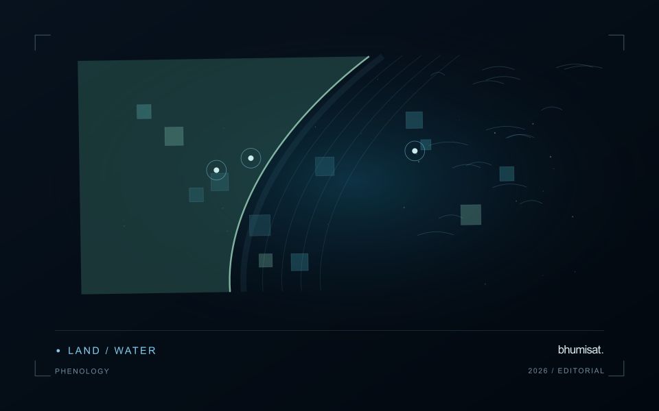
Mangrove monitoring takes place at a changing boundary between land and water. The observed surface depends on canopy structure, tidal conditions, exposed sediment and the arrangement of channels. A narrow fringe may contain a high proportion of mixed observations even when the surrounding image appears detailed. Begin by defining whether the task is mapping canopy extent, detecting disturbance or studying a forest attribute, and establish the spatial unit that the data can represent defensibly.
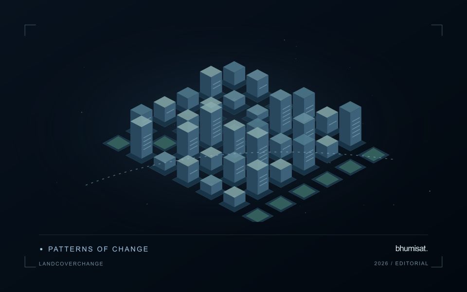
Comparisons between dates should account for water and sediment conditions as well as cloud, haze and shadow. A change near the canopy edge may reflect different water exposure or geometric alignment rather than a new loss of trees. Retain the acquisition dates and relevant tidal context where available. Mapping rules should distinguish canopy, water and other surfaces consistently, while acknowledging locations where their contributions cannot be separated reliably at the chosen resolution.
Field observations should describe canopy boundaries, vegetation structure and the setting of sampled plots or inspection points. Record whether a visit represents an edge, a channel margin or the forest interior. A mapped vegetation response alone cannot establish carbon stock, habitat quality or the cause of a disturbance. Those interpretations need suitable evidence. A practical initial product provides a traceable cover-change assessment and a prioritised set of locations where field review would resolve important uncertainty.
Define the quantity that the instrument records
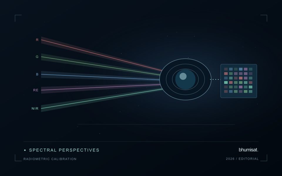
Radiometric calibration establishes a documented relationship between an instrument's recorded output and the physical quantity it is intended to represent. A stored pixel value may be a digital number, a scaled radiance or reflectance value, or another processed representation. Those alternatives should not be treated as interchangeable. The calibration chain explains how the recorded signal becomes an interpretable measurement and which corrections have already been applied. Understanding that chain is essential before comparing dates, combining bands or transferring a model between instruments.
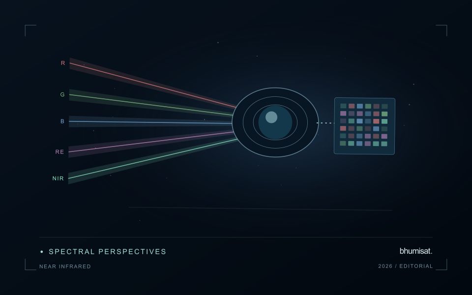
Instrument response can vary across detectors, channels and operating conditions. Calibration therefore concerns more than selecting one conversion coefficient. A study may need to consider offsets, response differences, noise, saturation and changes in behaviour over time. The appropriate characterisation depends on the instrument and its intended use. For a future payload concept, these are requirements to investigate rather than capabilities established by an attractive render. The presence of a multispectral camera alone does not demonstrate that its channels produce consistent, quantitatively comparable observations.
Track consistency through the complete chain
At the product level, begin with the supplier's definitions and metadata. Check scale factors, additive offsets, fill values and valid ranges before deriving an index or statistical summary. Preserve the processing version so that an output can be reproduced later. Inspect whether extreme values correspond to real surfaces or to invalid observations. When a dataset is updated, compare representative old and new results rather than assuming that a familiar file name guarantees an unchanged numerical meaning throughout the archive.
Validation should cover the full chain that supports the stated application. A stable response in a laboratory test is valuable evidence, while operational imagery introduces additional effects from atmosphere, geometry and scene complexity. Use independent references suited to the measurement scale and report the relevant uncertainty. Maintain a record of corrections and their limitations when delivering results to users. A traceable radiometric workflow supports meaningful comparisons and helps separate a change in the observation system from a change in the landscape that a monitoring service is trying to describe.
Check spatial alignment before comparison
A comparison between images, channels, maps, or field measurements assumes that the observations refer to the same locations at a suitable level of precision. Small alignment errors can become especially important near boundaries or narrow features. Before interpreting differences, inspect whether identifiable, stable features agree between the sources. A common coordinate reference is necessary for many workflows, but it does not by itself demonstrate accurate alignment.
Use control features that are appropriate for the observation scale and remain stable across the comparison period. Evaluate alignment in more than one part of the area, because a single location cannot reveal spatially varying distortion. Record the method used to estimate any correction and retain independent features for checking the corrected result. Where surfaces have genuinely changed, avoid using those changes as evidence of an alignment error.
Propagate the implications of remaining misalignment into the analysis. A workflow may exclude boundary pixels, summarise at a broader scale, or qualify interpretations for small features. The choice should follow the application rather than a preference for visually smooth output. Preserve both the original and corrected geographic references, and document resampling decisions so that future users can understand how measurements were moved onto a common spatial framework.
Design an evaluation that reflects deployment
A model evaluation should resemble the conditions in which the model will be used. Start by identifying which relationships the development data share: nearby locations, repeated observations of the same unit, common collection teams, or measurements from a single period. These relationships can make records less independent than they appear. An evaluation that ignores them may test the ability to recognise familiar conditions rather than the ability to operate in a new setting.
Choose a split strategy that matches the intended transfer. Holding out locations, seasons, operational units, or acquisition conditions can answer different questions. Document which question each split is designed to address, and keep the held-out evidence separate while selecting features and tuning the method. Repeatedly inspecting the same evaluation set to improve a model gradually makes that set part of development, even if it retains its original label.
Report results at a scale that is meaningful to the user. A strong average can hide poor performance for important subgroups or unusual conditions. Examine error patterns and retain examples of both successful and unsuccessful predictions. Where the evidence covers only a limited range of conditions, describe that range explicitly. The evaluation then becomes a practical guide to suitable use, further testing, and the collection of additional reference observations.
Bring the evidence back to the decision
A strong interpretation states what was observed, which explanations remain plausible, and what additional evidence would help distinguish them. Avoid presenting a convenient label as a confirmed cause when the measurements support only a broader pattern. Connect the proposed next step to the significance of the decision and the confidence available. This creates an interpretation that a field team, analyst, or project partner can examine, challenge, and improve as further observations become available.
Sources & further reading
Explore the bhumisat spacecraft concept and our vision towards 2030, or return to the journal.