Remote observations show patterns, while practical decisions depend on explaining what those patterns could mean. Interpretation therefore requires more than locating a high or low value on a map. A useful analysis considers the timing of the observation, the physical processes that influence the measurement, and the information available from complementary sources. This perspective separates an observed signal from a proposed explanation and from an action recommended to a user. Keeping those stages distinct makes it easier to investigate alternative causes, communicate ambiguity, and choose a proportionate next step.
This working guide considers how pointing and motion affect satellite imagery in open-field tomato production. The immediate decision is to select tomato rows for crop review. Useful reference evidence includes transplanting dates, canopy observations and field management notes. The case is an illustrative planning context, with assumptions to check against the actual sensor, landscape and project requirements.
The setting: Open-field tomato production
Open-field tomato production can involve short management cycles, staggered planting and repeated operations within neighbouring parcels. The field calendar is therefore central to interpreting a satellite observation. Newly transplanted plants, established rows and areas nearing the end of production can show different responses for ordinary reasons. Record the planted area and the relevant management unit carefully, particularly where a commercial holding contains several crops or planting stages at the same time.
The image footprint may mix plants with soil, mulch, access routes and irrigation infrastructure. Determine whether the spatial resolution supports the intended row-level interpretation or whether a broader field summary is more appropriate. Examine the quality and age of observations before proposing a management use that depends on rapid response. A monitoring workflow should communicate when cloud gaps or the acquisition schedule leave insufficient current evidence for that decision.
Validation should document crop stage, canopy continuity, recent operations and the area represented by each sample. Field staff may use a mapped anomaly to choose an inspection location, but the subsequent diagnosis requires suitable observations and expertise. If production or quality is the target, collect reference information for those outcomes rather than assuming that greener vegetation implies more marketable fruit. The evaluation should measure whether the product improves a defined scouting or management process.
Separate the different pointing requirements
A camera can point near its intended target while still producing an image with poor geometry or blur. Pointing accuracy describes how closely the spacecraft achieves a commanded orientation. Pointing knowledge describes how well that orientation is estimated. Stability concerns changes over a relevant interval, including the detector integration period. These quantities serve different purposes and should be specified separately with a clear reference frame and time basis.
Orientation estimates combine information from sensors such as gyroscopes, Sun sensors and star trackers, depending on the architecture. Actuators then change or maintain the attitude. Reaction wheels exchange angular momentum with the spacecraft, while magnetic torquers interact with Earth's magnetic field and may support momentum management. Their suitability depends on the orbit, operating modes and disturbance environment. A component's advertised accuracy does not automatically become the pointing performance of the integrated spacecraft.
Evaluate the complete image motion budget
Ground features move across a detector because the spacecraft travels along its orbit and may rotate during imaging. Exposure time, scan timing and any motion compensation must be consistent with that movement. Residual motion during integration spreads signal across pixels and reduces contrast. High frequency vibration can produce a different image effect from slow drift, so one average attitude error may conceal an important problem.
Build an image motion budget that includes control behavior, structural response, actuator disturbances and timing uncertainties. Consider the mechanical path between attitude sensors and the optical payload: a flexible interface can change their relative alignment. Thermal distortion can also alter boresight alignment over an orbit. Test realistic operating combinations, including wheel speeds and other mechanisms that may run during an exposure, and assess whether laboratory support equipment affects the measurement.
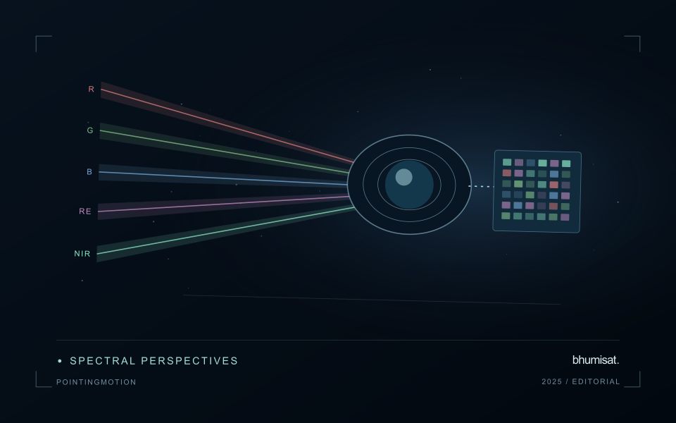
Geometric processing uses orbit information, attitude knowledge, timing and an Earth model to locate observations. Ground control and image matching can improve some errors, but processing cannot always restore information lost to blur. For repeat observations, test relative registration as well as absolute location. Report residual errors across the field and across relevant operating conditions. A useful requirement links a user consequence, such as registration between spectral bands, to a measurable spacecraft or payload behavior and a verification method. This keeps pointing discussions connected to the quality of the delivered imagery.
Represent gaps without inventing observations
A monitoring sequence often contains periods without a usable observation. The reason may be cloud, shadow, missing coverage, a failed transfer, or a quality condition that excludes the data. Begin by representing these states explicitly. A missing observation is different from a low measurement, an unchanged surface, or a confirmed absence of the feature being studied. The distinction should survive both the analysis and the presentation of the result.
Define when a temporal gap is acceptable for the intended decision. A workflow may continue using the latest qualified observation, request another source, or suspend an alert until sufficient evidence is available. Whichever response is selected, show the age of the supporting observation. If interpolation is used for a suitable analytical purpose, preserve the distinction between an estimated value and a directly observed measurement, together with the assumptions needed to interpret it.
Review how gaps affect the coverage of the final evaluation. Locations with frequent missing data may differ systematically from those with regular observations. A performance estimate based only on clear, complete records can therefore describe a narrower population than the service is expected to support. Report usable coverage alongside analytical results and use recurring gaps to guide acquisition planning, reference collection, and the selection of complementary observation methods.
Plan the evidence needed for calibration
Calibration connects an instrument's recorded response with a measurement that can be interpreted consistently. Begin by identifying which aspects of the response matter to the application: variation across channels, changes with operating conditions, geometric alignment, or differences between repeated observations. A calibration plan should state the quantities being assessed and the evidence needed to determine whether the response is sufficiently characterised for the intended use.
Design tests around controlled and documented conditions. Record the reference source, instrument configuration, exposure settings, temperature conditions, and processing applied to the measurements. Repeat suitable observations to investigate variability and distinguish a consistent response from a single favourable result. The reference itself has limitations, so preserve its characterisation and avoid assuming that every difference originates in the instrument under evaluation.
Connect calibration activities with the expected operating environment and processing chain. A correction that works under one test condition may require further evidence before being applied elsewhere. Define how calibration parameters are versioned, checked, and associated with the observations they support. Include a plan for recognising drift or other changes that could affect interpretation. The outcome should be an instrument response supported by traceable evidence, together with acceptance criteria that remain relevant to the application.
Bring the evidence back to the decision
A strong interpretation states what was observed, which explanations remain plausible, and what additional evidence would help distinguish them. Avoid presenting a convenient label as a confirmed cause when the measurements support only a broader pattern. Connect the proposed next step to the significance of the decision and the confidence available. This creates an interpretation that a field team, analyst, or project partner can examine, challenge, and improve as further observations become available.
Sources & further reading
Explore the bhumisat spacecraft concept and our vision towards 2030, or return to the journal.