Every observation and interpretation contains uncertainty, but the sources and consequences of that uncertainty differ between applications. Some arise from acquisition conditions, others from reference measurements, processing choices, or the transfer of a model to a new setting. This perspective examines how those sources affect the decision a user is considering. It encourages teams to describe uncertainty in a form that can influence action, rather than adding a generic qualification at the end of a report. The objective is to support proportionate decisions while keeping the limits of the available evidence understandable.
This working guide considers satellite time series and crop phenology in sugarcane production blocks. The immediate decision is to sequence scouting and harvest review. Useful reference evidence includes planting or ratoon dates and dated canopy observations. The case is an illustrative planning context, with assumptions to check against the actual sensor, landscape and project requirements.
The setting: Sugarcane production blocks
Sugarcane monitoring depends on knowing where each block sits within a management cycle. A recently planted field, an established ratoon and a block approaching harvest can have very different canopy structures without any of them indicating a problem. Maintain planting and harvest dates alongside block boundaries, and distinguish crop establishment from regrowth. This context gives a time series a meaningful starting point and prevents comparisons between fields at unrelated stages.
A useful workflow follows the development of each block through successive quality-screened observations. Look for departures from comparable blocks or from a documented local seasonal pattern, rather than applying a single threshold across the whole estate. Harvest operations, residue management, bare soil and weeds can all affect the surface signal. Track these events in the same record as the imagery so that the analytical timeline reflects what actually happened on the ground.
Field validation should address a defined question, such as whether a flagged area has uneven establishment or requires an agronomic visit. Record crop stage, stand continuity, management history and the location of observations within the block. Predictions related to production need suitable harvest measurements and evaluation across seasons. A map that helps organise scouting is useful evidence of a workflow; it is not automatically a validated estimate of cane tonnage.
Describe a seasonal trajectory
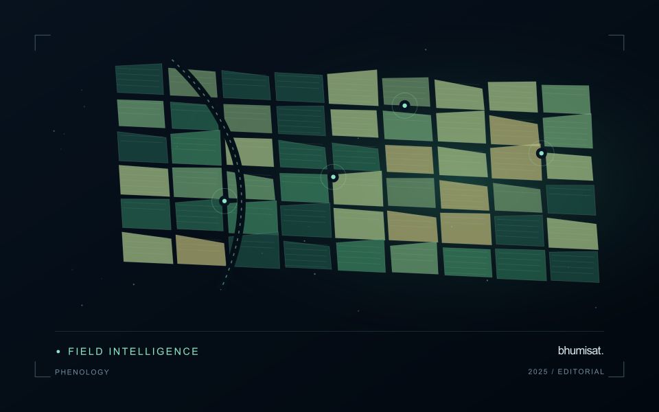
Phenology concerns the timing of recurring biological development. In an agricultural image series, a changing canopy can create a trajectory associated with establishment, growth, maturity and harvest. The trajectory is an indirect observation of those processes. Satellite measurements do not necessarily identify each agronomic stage on their own. A useful interpretation connects the series with crop type, planting information and field observations. This helps distinguish an unexpected development pattern from a normal difference in variety, management or seasonal timing.
The first design choice is the unit of comparison. A management block, planting cohort or crop zone may provide a more meaningful series than a broad administrative area containing several crops. Keep the spatial unit consistent and track changes to its boundary. Record which summary statistic is used and how many valid observations support it. A smooth line can be visually persuasive even when it connects only a few reliable dates. The chart should make gaps and uncertain periods visible instead of implying continuous knowledge.
Evaluate timing and missing observations
Timing metrics require explicit definitions. The date of a measured increase, the date inferred from a fitted curve and the date recorded by a field team may differ. Decide which quantity is needed and how it will be evaluated. Smoothing can reduce noise, but an overly flexible or overly rigid method can alter the apparent timing of an event. Compare candidate settings against independent observations and inspect whether they behave sensibly during short seasons, interrupted growth and abrupt management changes.
A practical monitoring service also needs a policy for delayed and missing data. Optical cloud cover can obscure a critical part of a season, and a later observation may only confirm that a transition occurred within an interval. Report that interval where appropriate. Do not replace an unavailable observation with an unlabelled estimate. Over several seasons, evaluate whether the derived timing information improves planning or interpretation and whether the relationship remains stable. The goal is a defensible seasonal description that supports a field decision, with its temporal uncertainty retained.
Represent gaps without inventing observations
A monitoring sequence often contains periods without a usable observation. The reason may be cloud, shadow, missing coverage, a failed transfer, or a quality condition that excludes the data. Begin by representing these states explicitly. A missing observation is different from a low measurement, an unchanged surface, or a confirmed absence of the feature being studied. The distinction should survive both the analysis and the presentation of the result.
Define when a temporal gap is acceptable for the intended decision. A workflow may continue using the latest qualified observation, request another source, or suspend an alert until sufficient evidence is available. Whichever response is selected, show the age of the supporting observation. If interpolation is used for a suitable analytical purpose, preserve the distinction between an estimated value and a directly observed measurement, together with the assumptions needed to interpret it.
Review how gaps affect the coverage of the final evaluation. Locations with frequent missing data may differ systematically from those with regular observations. A performance estimate based only on clear, complete records can therefore describe a narrower population than the service is expected to support. Report usable coverage alongside analytical results and use recurring gaps to guide acquisition planning, reference collection, and the selection of complementary observation methods.
Budget the complete processing workflow
A processing budget should cover the complete path from source observations to a maintained product. Data access and computing are only part of that path. Include preparation, geographic updates, reference collection, expert review, delivery, and support where those activities belong to the service. A calculation that runs cheaply on a small demonstration can still require substantial effort when the surrounding work is repeated across many locations.
Measure representative tasks rather than assuming that every observation costs the same amount to process. Record data volume, processing time, retry frequency, manual interventions, and the conditions that create unusually demanding cases. Separate fixed setup work from work that grows with the number of observations or users. These records support decisions about batching, caching, storage policy, and the point at which a different processing design becomes worthwhile.
Connect the budget to a defined level of service. Faster delivery, more frequent observation, broader coverage, or more detailed review can each change the resources required. Describe these trade-offs before promising a delivery pattern that the workflow has not demonstrated. Review the budget using operational evidence and preserve enough detail to understand changes between processing versions. The aim is a sustainable service whose resource choices remain aligned with the information that users value.
Bring the evidence back to the decision
Useful uncertainty communication identifies the limitation, explains how it could affect the result, and connects it to a practical response. Some decisions can proceed with a qualified estimate; others require another observation or an independent check. Preserve uncertainty information through processing and delivery so that it is available at the point of use. This makes the analysis more accountable and gives the team a clearer basis for deciding which additional evidence would most improve the outcome.
Sources & further reading
Explore the bhumisat spacecraft concept and our vision towards 2030, or return to the journal.