Comparisons through time are valuable only when the observations are sufficiently comparable for the question being asked. A difference between dates can reflect real change, a normal stage in a seasonal cycle, or a difference in how the surface was observed. This perspective examines the reference period, the timing of acquisitions, and the contextual records needed to interpret a sequence. It encourages the use of appropriate baselines rather than treating every previous observation as an equivalent benchmark. The objective is to identify changes that remain meaningful after normal variation and measurement conditions are considered.
This working guide considers near-infrared observations of vegetation and land in onion production beds. The immediate decision is to review beds with uneven establishment. Useful reference evidence includes planting dates, bed cover and crop-stage observations. The case is an illustrative planning context, with assumptions to check against the actual sensor, landscape and project requirements.
The setting: Onion production beds
Onion fields can retain a strong soil contribution in optical imagery because of their canopy form and the arrangement of production beds. The proportion of exposed soil, the stage of the crop and the condition of neighbouring surfaces all matter to interpretation. A useful monitoring design begins by identifying whether it needs a field-level development indicator or more detailed bed-level information. The image data must genuinely support the scale at which conclusions are presented.
Maintain planting and management records alongside the image sequence, and distinguish normal stage differences from unusual spatial patterns. Small fields may contain only a limited number of observations that are not mixed with boundaries, tracks or other crops. Quality screening should account for this limitation rather than treating every nominal pixel as an independent view of onions. Comparable acquisition and processing conditions strengthen the interpretation of changes between reporting periods.
Field visits should record crop stage, stand continuity and the condition of the soil and bed surfaces contributing to the image. Sample across the mapped range, including areas that look typical, and preserve the location and date of each observation. A general reflectance pattern cannot directly establish bulb production or a named cause of stress. Those claims need appropriate measurements, while a transparent inspection-priority workflow can be evaluated through the outcomes of practical scouting visits.
Understand what contributes to the NIR response
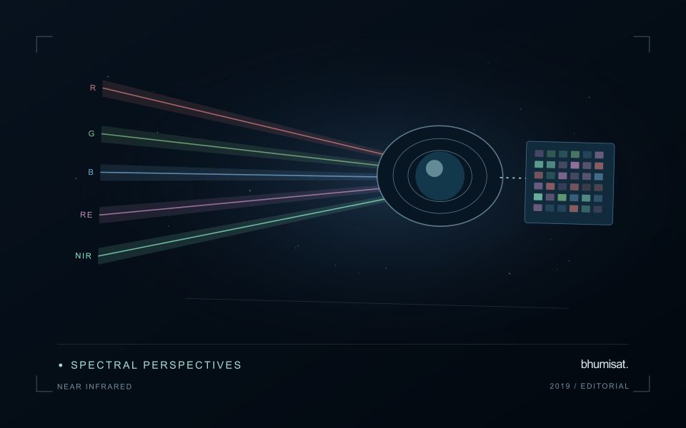
Near-infrared wavelengths lie outside the range of human vision, but they are important in optical observations of vegetation and land. A near-infrared image should not be confused with a thermal image. Reflected sunlight in this region and emitted thermal radiation describe different physical processes. This distinction matters when communicating crop information: a bright or dark NIR response is not a direct temperature reading. Its interpretation depends on the surface, the observation geometry and the particular wavelength interval measured by the instrument.
Vegetation can show a strong near-infrared response because of interactions within leaves and canopies. At landscape scale, the observed signal also changes with canopy cover, leaf arrangement, shadows and the proportion of visible soil or water. A field with a different crop age may therefore differ substantially from another field without either being abnormal. NIR is useful partly because it adds contrast beyond visible appearance, but that contrast still needs a meaningful comparison. The analytical task determines which associated measurements and field records are required.
Use NIR in a traceable analytical chain
When combining NIR with another band in an index or model, check that the channels refer to comparable ground locations and acquisition conditions. Differences in band resolution, alignment or spectral response can influence the result. Preserve reflectance scale factors, quality flags and any processing applied before the combination. Where resampling is necessary, choose a documented common grid and recognise that the operation changes representation rather than increasing the original observation detail. These controls are particularly important near field edges and in small management units.
An application should demonstrate the benefit of the NIR measurement using evidence appropriate to its stated purpose. For vegetation monitoring, that might mean a relationship with independently recorded canopy conditions or a reliable separation of relevant land-cover classes. For water or soil interpretation, a different protocol may be needed. Review errors as well as successful examples and retain cases that challenge the initial explanation. A clear observation chain makes NIR a useful part of a broader decision process without assigning the band capabilities it does not independently provide.
Check spatial alignment before comparison
A comparison between images, channels, maps, or field measurements assumes that the observations refer to the same locations at a suitable level of precision. Small alignment errors can become especially important near boundaries or narrow features. Before interpreting differences, inspect whether identifiable, stable features agree between the sources. A common coordinate reference is necessary for many workflows, but it does not by itself demonstrate accurate alignment.
Use control features that are appropriate for the observation scale and remain stable across the comparison period. Evaluate alignment in more than one part of the area, because a single location cannot reveal spatially varying distortion. Record the method used to estimate any correction and retain independent features for checking the corrected result. Where surfaces have genuinely changed, avoid using those changes as evidence of an alignment error.
Propagate the implications of remaining misalignment into the analysis. A workflow may exclude boundary pixels, summarise at a broader scale, or qualify interpretations for small features. The choice should follow the application rather than a preference for visually smooth output. Preserve both the original and corrected geographic references, and document resampling decisions so that future users can understand how measurements were moved onto a common spatial framework.
Plan the evidence needed for calibration
Calibration connects an instrument's recorded response with a measurement that can be interpreted consistently. Begin by identifying which aspects of the response matter to the application: variation across channels, changes with operating conditions, geometric alignment, or differences between repeated observations. A calibration plan should state the quantities being assessed and the evidence needed to determine whether the response is sufficiently characterised for the intended use.
Design tests around controlled and documented conditions. Record the reference source, instrument configuration, exposure settings, temperature conditions, and processing applied to the measurements. Repeat suitable observations to investigate variability and distinguish a consistent response from a single favourable result. The reference itself has limitations, so preserve its characterisation and avoid assuming that every difference originates in the instrument under evaluation.
Connect calibration activities with the expected operating environment and processing chain. A correction that works under one test condition may require further evidence before being applied elsewhere. Define how calibration parameters are versioned, checked, and associated with the observations they support. Include a plan for recognising drift or other changes that could affect interpretation. The outcome should be an instrument response supported by traceable evidence, together with acceptance criteria that remain relevant to the application.
Bring the evidence back to the decision
A useful comparison preserves the dates, quality conditions, and contextual assumptions behind its baseline. Review unusual results against the actual observation sequence rather than relying entirely on a summary statistic. Where seasonal timing is important, describe how comparable stages were identified. The resulting analysis should help users distinguish an informative change from an expected cycle or an observation artefact, while making gaps and remaining uncertainty visible enough to guide further investigation.
Sources & further reading
Explore the bhumisat spacecraft concept and our vision towards 2030, or return to the journal.