Comparisons through time are valuable only when the observations are sufficiently comparable for the question being asked. A difference between dates can reflect real change, a normal stage in a seasonal cycle, or a difference in how the surface was observed. This perspective examines the reference period, the timing of acquisitions, and the contextual records needed to interpret a sequence. It encourages the use of appropriate baselines rather than treating every previous observation as an equivalent benchmark. The objective is to identify changes that remain meaningful after normal variation and measurement conditions are considered.
This working guide considers ndvi crop monitoring in maize production fields. The immediate decision is to prioritise uneven-development scouting. Useful reference evidence includes emergence dates, plant stand notes and field stage. The case is an illustrative planning context, with assumptions to check against the actual sensor, landscape and project requirements.
What the index can describe
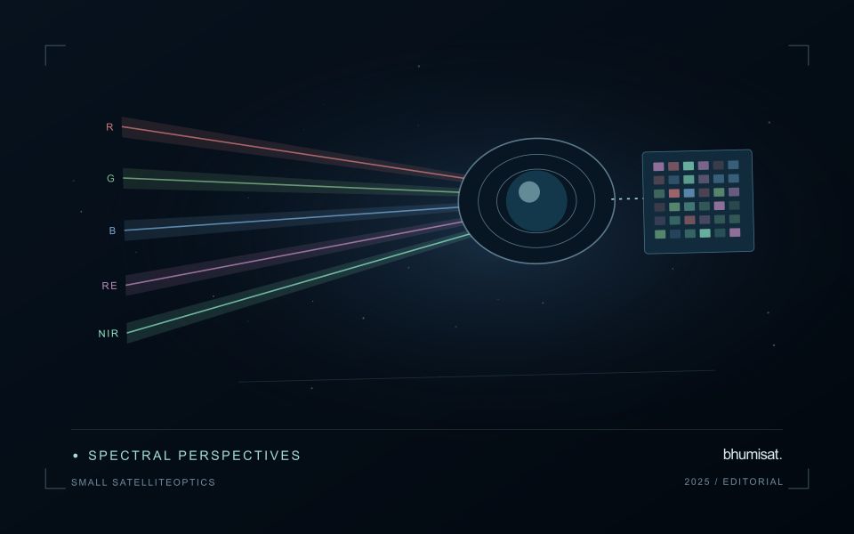
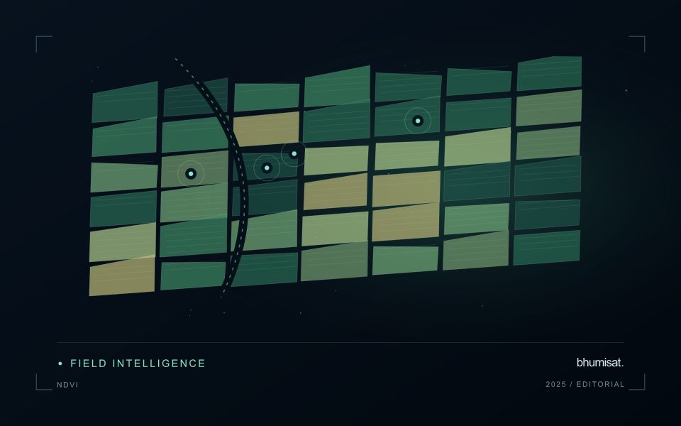
NDVI expresses the contrast between near-infrared and red reflectance as their difference divided by their sum. The result is a compact description of spectral behaviour, rather than a direct measurement of crop health. A growing canopy often changes both of these measurements, but soil exposure, standing water, illumination and the mixture of materials inside a pixel can also affect the index. An operational interpretation therefore starts with the crop, its development stage and the surface actually represented by the pixels.
A useful monitoring baseline describes comparable conditions. Comparing a newly planted field with an older field can produce a strong difference that simply reflects age. Comparing the same field before and after harvest can be useful if the management record confirms the event. The analytical question should be stated before choosing an alert threshold: detecting an unexpected departure from normal development is different from mapping current canopy cover. Neither task automatically establishes the cause of a low value or the action a grower should take.
Build a comparison that can be checked
Before computing field statistics, screen unsuitable observations and retain their quality information. The processing record should identify the imagery source, acquisition date, reflectance product, band mapping and mask rules. Report how much valid area remains inside each field. A median calculated from a small cloud-free corner should not be presented as if it represented the entire management block. Keeping a distribution or selected percentiles alongside the central value can reveal variation that a single coloured label would hide from the user.
Validation should connect an apparent change with an independent observation at a relevant time. A field team can record canopy condition, crop stage, recent operations and any visible disturbance, including observations that contradict the alert. Revisit both flagged and apparently normal areas to evaluate missed changes and false alarms. Once a relationship has been demonstrated, monitor whether it remains stable across seasons and management systems. NDVI is most useful when it helps organise a defensible comparison and directs attention to places where additional information is needed.
The setting: Maize production fields
Maize fields can differ in emergence date, variety, plant density and management even within the same growing region. An image comparison is more meaningful when those differences are recorded. Early in the cycle, visible soil and row arrangement can influence a field summary substantially. Later, the canopy may become dense enough that some vegetation measures respond less clearly to additional growth. Interpret the observations in relation to the crop stage and the variable of interest.
Construct a field timeline that marks establishment, important field operations and the dates of usable observations. A decline or delayed increase in a signal can suggest a place to investigate, but several explanations may be possible. Soil conditions, weeds, storm effects and crop timing can produce patterns that require field context. Avoid turning a general anomaly map into a specific diagnosis without measurements that distinguish between these alternatives.
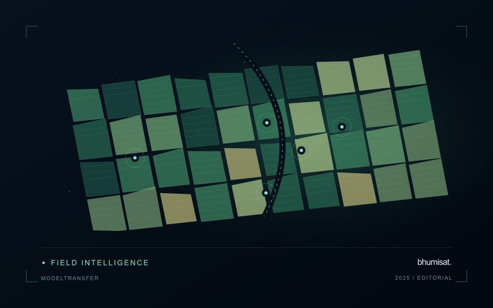
A scouting plan should include representative normal areas as well as the locations ranked most unusual. Record crop stage, stand continuity, visible damage and management information consistently. Production models require their own training and evaluation data, ideally covering different fields and seasons. For operational use, assess whether a satellite-derived priority list helps the field team find relevant conditions efficiently, and report the observation age whenever weather leaves a gap in the current image sequence.
Design an evaluation that reflects deployment
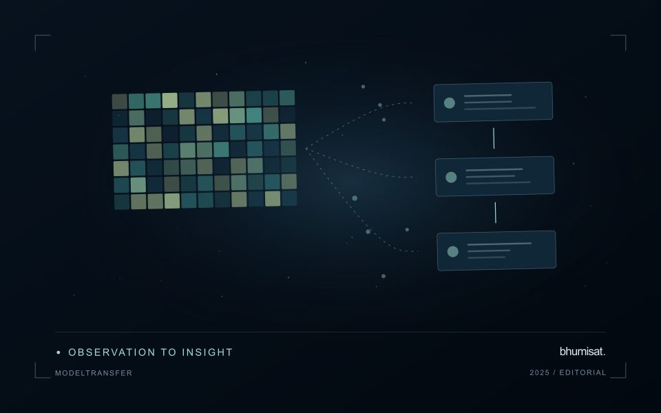
A model evaluation should resemble the conditions in which the model will be used. Start by identifying which relationships the development data share: nearby locations, repeated observations of the same unit, common collection teams, or measurements from a single period. These relationships can make records less independent than they appear. An evaluation that ignores them may test the ability to recognise familiar conditions rather than the ability to operate in a new setting.
Choose a split strategy that matches the intended transfer. Holding out locations, seasons, operational units, or acquisition conditions can answer different questions. Document which question each split is designed to address, and keep the held-out evidence separate while selecting features and tuning the method. Repeatedly inspecting the same evaluation set to improve a model gradually makes that set part of development, even if it retains its original label.
Report results at a scale that is meaningful to the user. A strong average can hide poor performance for important subgroups or unusual conditions. Examine error patterns and retain examples of both successful and unsuccessful predictions. Where the evidence covers only a limited range of conditions, describe that range explicitly. The evaluation then becomes a practical guide to suitable use, further testing, and the collection of additional reference observations.
Translate the decision into observation requirements
Start with the decision that the information is intended to support. Describe the geographic unit, the time available for acting, and the consequence of an incorrect interpretation. A requirement such as detecting an unusual pattern across management blocks is different from identifying its cause. Keeping that distinction explicit helps a team select measurements that are relevant to the application and prevents later evaluation from drifting towards whatever result happens to be easiest to demonstrate.
Build a compact requirements matrix linking each decision to the evidence needed, the proposed observation source, and an acceptance condition. Include geographic accuracy, temporal relevance, quality screening, and the context required for interpretation. The matrix should also identify the evidence used to justify each requirement. An engineering preference or a convenient data source can inform a study, but neither should silently replace a documented information need.
Review the matrix with the people who will use the result. Ask how their response would change when information is delayed, incomplete, or uncertain. Record unresolved requirements as questions for a pilot rather than converting them into confident specifications. This produces a practical framework for comparing technical options, designing tests, and explaining why an observation is useful to the intended workflow.
Bring the evidence back to the decision
A useful comparison preserves the dates, quality conditions, and contextual assumptions behind its baseline. Review unusual results against the actual observation sequence rather than relying entirely on a summary statistic. Where seasonal timing is important, describe how comparable stages were identified. The resulting analysis should help users distinguish an informative change from an expected cycle or an observation artefact, while making gaps and remaining uncertainty visible enough to guide further investigation.
Sources & further reading
Explore the bhumisat spacecraft concept and our vision towards 2030, or return to the journal.