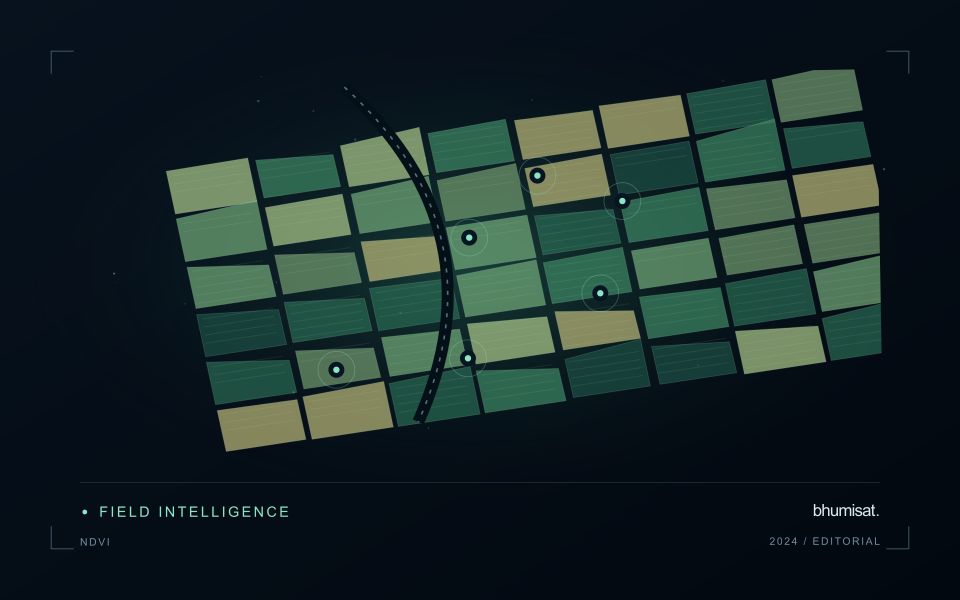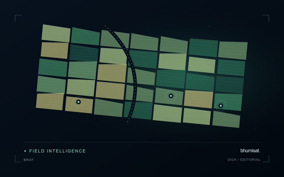
Comparisons through time are valuable only when the observations are sufficiently comparable for the question being asked. A difference between dates can reflect real change, a normal stage in a seasonal cycle, or a difference in how the surface was observed. This perspective examines the reference period, the timing of acquisitions, and the contextual records needed to interpret a sequence. It encourages the use of appropriate baselines rather than treating every previous observation as an equivalent benchmark. The objective is to identify changes that remain meaningful after normal variation and measurement conditions are considered.
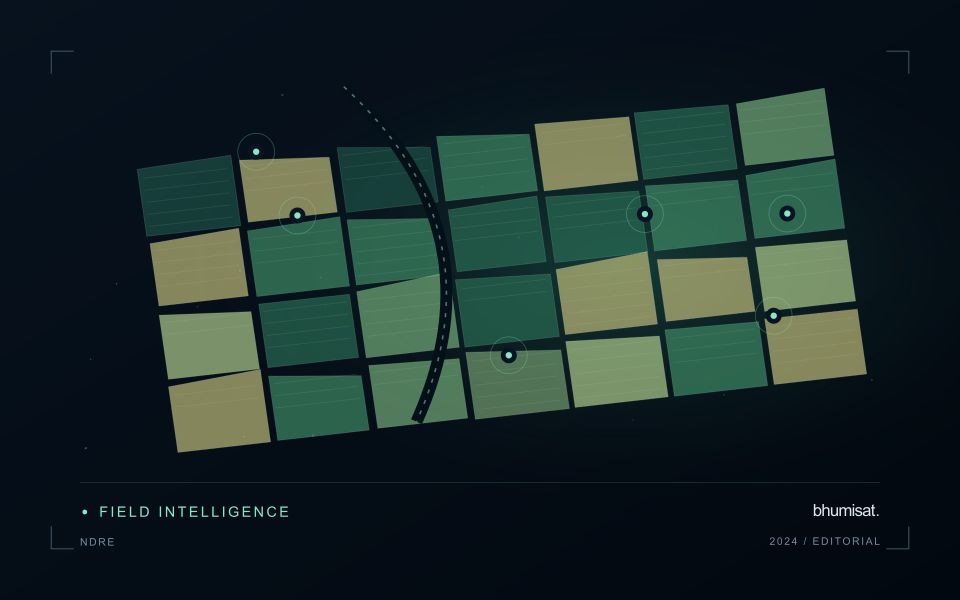
This working guide considers ndre and crop canopy interpretation across coconut production landscapes. The immediate decision is to identify areas needing plantation review. Useful reference evidence includes palm spacing, understory condition and farm-level observations. The case is an illustrative planning context, with assumptions to check against the actual sensor, landscape and project requirements.
Define the Red Edge measurement precisely
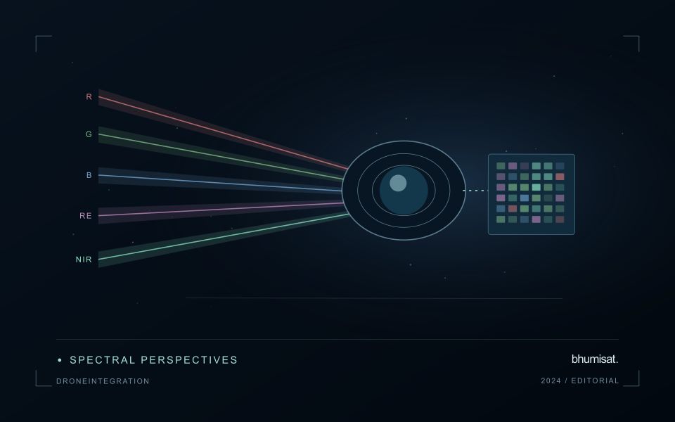
NDRE uses the contrast between near-infrared reflectance and a selected Red Edge band, commonly expressed as a normalised difference. Its meaning depends on the actual spectral response of those channels. Two instruments described as having Red Edge capability may observe different wavelength intervals, so their index values are not automatically interchangeable. Record the selected bands, the product level and any resampling applied to them. This is particularly important when a monitoring service combines observations from several satellite or aerial instruments.
The Red Edge region captures a transition between strong absorption in red wavelengths and the higher reflectance often observed in near-infrared wavelengths over vegetation. A measurement in that transition can provide information that differs from a conventional red band. However, canopy structure, growth stage, soil visibility and illumination also influence the observed signal. An apparent improvement over another index should be demonstrated for a defined crop parameter and evaluation dataset, rather than inferred from the presence of an additional spectral channel alone.
Separate spectral sensitivity from agronomic evidence
A sound comparison uses compatible surface reflectance inputs and observations of similar quality. Inspect cloud edges, shadows, band alignment and field boundaries before interpreting small changes. Bands with different native spatial sampling may require a common grid, but resampling does not create new measured ground detail. Where the field contains only a few usable pixels, boundary mixing can dominate the result. Summarising an interior area separately from the full field can help reveal that sensitivity, provided the exclusion rule is documented consistently.
An agricultural model built around NDRE needs independent measurements of the parameter it claims to estimate. If the objective concerns leaf or canopy condition, the field protocol should specify what is measured, where, when and at what scale. Keep calibration observations separate from the final evaluation sample. Examine performance across crop ages and management regimes, including difficult cases. The resulting evidence can support a targeted application, while uncertainty and sampling limits remain visible. A spectral response is an observation; an agronomic conclusion requires an additional, tested relationship.
The setting: Coconut production landscapes
Coconut production landscapes can range from organised plantations to widely spaced palms embedded in farms, settlements and coastal vegetation. These settings create very different observation problems. A satellite pixel may combine palm crowns, soil, grass, roofs or water rather than represent coconut vegetation alone. Define whether the task is mapping a production landscape, documenting canopy change or studying a crop-specific variable before choosing an image product or interpretation method.
Field and management boundaries are important even where ownership units do not coincide with a continuous canopy. Record the extent of intercropping and other vegetation that may contribute to an observed change. In coastal settings, inspect shoreline adjacency, temporary flooding and atmospheric conditions alongside the imagery. A field-average vegetation response should be accompanied by the area and quality of the observations from which it was calculated.
Validation should describe palm arrangement, canopy continuity, understory and recent land-management events at known locations. Samples drawn only from dense or easily accessible stands may not represent the wider landscape. A model intended for crop condition or production needs reference measurements suited to that claim and evaluation beyond its development sites. For many users, a transparent inventory and a well-supported list of locations requiring review provide a practical foundation for later, more specialised analytical services.
Maintain the geographic units of analysis
Many observation services summarise measurements within a field, management block, catchment, forest unit, or other mapped boundary. The meaning of that summary depends on whether the boundary accurately represents the unit being discussed. Start with a clear source for the geometry and record its date, coordinate reference, and intended use. A boundary drawn for visual orientation may require additional checking before it becomes a measurement unit.
Inspect overlaps, gaps, narrow fragments, and features that may have changed since mapping. A geometrically valid polygon can still describe an outdated operational unit. Ask the responsible team how divisions, mergers, new infrastructure, and management changes are recorded. Where pixels or reference measurements cross a boundary, define how they are assigned or excluded so that results remain comparable between analysts and processing runs.
Version the boundaries alongside the observations. If a unit changes, preserve a relationship between the previous and revised geometry rather than replacing the history without explanation. Comparisons through time should identify whether they use a constant spatial unit or the operational units valid at each date. This makes it easier to distinguish a change in the measured surface from a change introduced by the geography used to summarise it.
Represent gaps without inventing observations
A monitoring sequence often contains periods without a usable observation. The reason may be cloud, shadow, missing coverage, a failed transfer, or a quality condition that excludes the data. Begin by representing these states explicitly. A missing observation is different from a low measurement, an unchanged surface, or a confirmed absence of the feature being studied. The distinction should survive both the analysis and the presentation of the result.
Define when a temporal gap is acceptable for the intended decision. A workflow may continue using the latest qualified observation, request another source, or suspend an alert until sufficient evidence is available. Whichever response is selected, show the age of the supporting observation. If interpolation is used for a suitable analytical purpose, preserve the distinction between an estimated value and a directly observed measurement, together with the assumptions needed to interpret it.
Review how gaps affect the coverage of the final evaluation. Locations with frequent missing data may differ systematically from those with regular observations. A performance estimate based only on clear, complete records can therefore describe a narrower population than the service is expected to support. Report usable coverage alongside analytical results and use recurring gaps to guide acquisition planning, reference collection, and the selection of complementary observation methods.
Bring the evidence back to the decision
A useful comparison preserves the dates, quality conditions, and contextual assumptions behind its baseline. Review unusual results against the actual observation sequence rather than relying entirely on a summary statistic. Where seasonal timing is important, describe how comparable stages were identified. The resulting analysis should help users distinguish an informative change from an expected cycle or an observation artefact, while making gaps and remaining uncertainty visible enough to guide further investigation.
Sources & further reading
Explore the bhumisat spacecraft concept and our vision towards 2030, or return to the journal.