Comparisons through time are valuable only when the observations are sufficiently comparable for the question being asked. A difference between dates can reflect real change, a normal stage in a seasonal cycle, or a difference in how the surface was observed. This perspective examines the reference period, the timing of acquisitions, and the contextual records needed to interpret a sequence. It encourages the use of appropriate baselines rather than treating every previous observation as an equivalent benchmark. The objective is to identify changes that remain meaningful after normal variation and measurement conditions are considered.
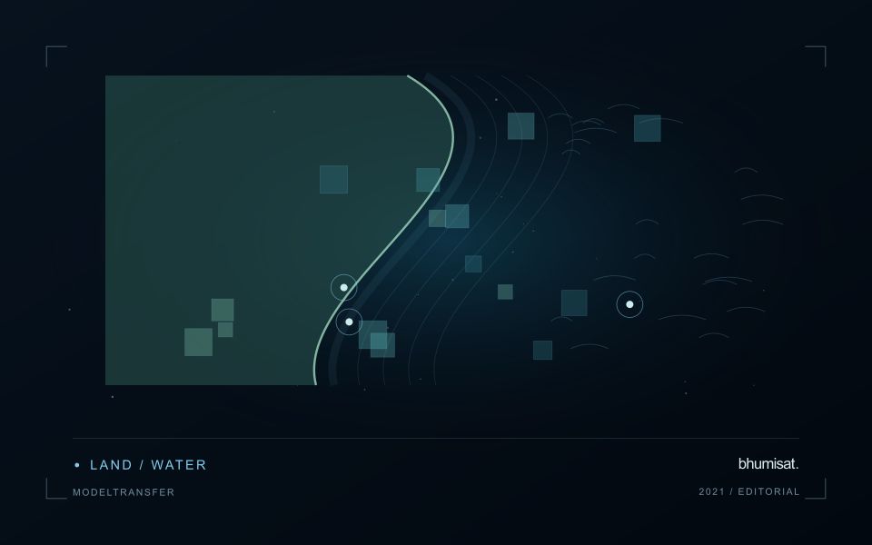
This working guide considers testing whether a remote sensing model transfers along river water corridors. The immediate decision is to prioritise river reaches for sampling. Useful reference evidence includes sampling time, river stage and reach-specific water observations. The case is an illustrative planning context, with assumptions to check against the actual sensor, landscape and project requirements.
The setting: River water corridors
A river corridor can vary quickly in width, bank exposure, flow conditions and the surrounding land cover. A remotely observed reach may include water, sediment, vegetation and structures within the same footprint. Define the monitoring question before choosing an interpretation scale. Mapping the position of visible water, investigating a colour change and estimating a particular water-quality variable are different tasks, even where they draw on the same acquisition.
Spatial resolution and geometric alignment are critical for narrow reaches. A small offset can change how much bank or vegetation contributes to a measurement. Cloud, shadow, surface reflection and adjacency effects can further complicate optical interpretation. Compare suitable acquisitions and retain the exact dates supporting each reach summary. Where river conditions change rapidly, consider whether the available observation frequency is sufficient for the decision the service is intended to support.
Field sampling should identify the sampled reach, location and collection time, together with river conditions that affect comparability. A single bank-side sample may not describe the full width or a downstream reach observed at another time. A spectral anomaly can help select an investigation site without establishing its cause. More specific claims require a validated relationship with representative measurements, while a transparent water and reach inventory can already make a sampling programme more systematic.
Identify what changes between domains
A model trained on one region or season learns relationships present in its development data. Applying it elsewhere assumes those relationships remain useful. New crop varieties, forest types, soil colours, management practices, illumination, or sensor characteristics can violate that assumption. Define the intended transfer explicitly: a new district, another year, another sensor, or a different class distribution. Each change creates a different test. A model that transfers across nearby fields has not thereby demonstrated reliable performance across climates or observation systems.
Keep the measurement pipeline consistent before attributing differences to the model. Reflectance scaling, band order, cloud masking, spatial resolution, composite windows, and missing value handling can all change predictions. Sensors with similarly named bands may have different spectral responses. Harmonization can reduce some differences but does not establish equivalence for every target. Examine predictor distributions, missing data rates, and examples from the new setting. Flag inputs outside the conditions represented during training so that extrapolation remains visible.
Test the destination, then adapt carefully
Design evaluation splits around the intended deployment. Hold out geographic regions to test spatial transfer and later years to test temporal transfer, keeping neighboring samples or repeated observations of the same site together when needed. Report performance for meaningful destination groups rather than only a pooled score. Class prevalence affects some metrics, so interpret changes alongside the underlying confusion matrix or residual distributions. A random pixel split can look excellent while providing little evidence about performance in an unseen region.
If local labels are available, reserve a destination assessment set before fine tuning or recalibration. Use the remaining observations to compare straightforward baselines with more complex adaptation methods. Check whether improvement comes from genuine transfer or simply from adding representative local data. Retain an option to withhold predictions when input quality or novelty makes them unreliable. Document the training domain, destination evidence, preprocessing versions, and conditions where use is unsupported. Continue monitoring once new observations arrive, since seasonal and environmental shifts can emerge after an initial evaluation. Transferability is a measured property of a particular model, workflow, target, and destination; it should not be inferred from architecture name or strong performance on the original test set.
Organise imagery and results for reliable retrieval
A useful storage design helps people and software find the right observation without relying on informal knowledge of folder names. Separate immutable source data from temporary processing files and delivered products. Give each observation a stable identifier and preserve its acquisition metadata alongside the file. A predictable organisation reduces the chance that a later analysis accidentally uses a preview, an outdated result, or an intermediate product whose meaning has not been documented.
Choose an indexing scheme that reflects the questions the workflow needs to answer. Location, acquisition time, source, product type, and processing version are often useful search dimensions. The physical arrangement of files can differ from the logical catalogue, provided that the relationship is maintained reliably. Record checksums or other integrity information where appropriate, and test whether an observation can be recovered using the catalogue rather than a particular operator's memory.
Define retention rules for source, intermediate, and delivered information. Some intermediate products are inexpensive to reproduce, while others embody costly preparation or expert review. Keep the inputs and configuration needed to rebuild a result before removing reproducible files. Test backup and recovery procedures with representative products, including their metadata and geographic references. Reliable retrieval is demonstrated by a successful reconstruction of useful information, rather than by the existence of an untested copy.
Establish a metadata contract
Define a small set of metadata that every observation and derived product must carry through the workflow. Useful fields include a stable identifier, acquisition time, geographic reference, spatial coverage, measurement units, source version, and processing status. The purpose is not to collect every possible detail. It is to preserve the information required to interpret, compare, locate, and reproduce the observations that the application depends on.
Specify field names, allowed formats, and the meaning of missing values. A blank field, a value of zero, and a measurement below a detection threshold are different states and should remain distinguishable. Time zones, coordinate order, and unit conversions deserve particular attention because inconsistent conventions can produce plausible-looking results that are difficult to diagnose. Validate the metadata when information enters the system, while the source and collection context remain available.
Treat the metadata contract as part of the delivery interface. A product passed to another team should retain the identifiers needed to trace its source and processing history. If a transformation changes the meaning of a field, create a new field or document the change rather than reusing the original name silently. A clear contract reduces ambiguity between field collectors, analysts, software components, and the eventual users of the information.
Bring the evidence back to the decision
A useful comparison preserves the dates, quality conditions, and contextual assumptions behind its baseline. Review unusual results against the actual observation sequence rather than relying entirely on a summary statistic. Where seasonal timing is important, describe how comparable stages were identified. The resulting analysis should help users distinguish an informative change from an expected cycle or an observation artefact, while making gaps and remaining uncertainty visible enough to guide further investigation.
Sources & further reading
Explore the bhumisat spacecraft concept and our vision towards 2030, or return to the journal.