Remote observations show patterns, while practical decisions depend on explaining what those patterns could mean. Interpretation therefore requires more than locating a high or low value on a map. A useful analysis considers the timing of the observation, the physical processes that influence the measurement, and the information available from complementary sources. This perspective separates an observed signal from a proposed explanation and from an action recommended to a user. Keeping those stages distinct makes it easier to investigate alternative causes, communicate ambiguity, and choose a proportionate next step.
This working guide considers testing whether a remote sensing model transfers across periurban land transitions. The immediate decision is to review changing land-use boundaries. Useful reference evidence includes dated land-use observations and parcel-level reference records. The case is an illustrative planning context, with assumptions to check against the actual sensor, landscape and project requirements.
The setting: Periurban land transitions
A periurban landscape can contain agricultural fields, new buildings, open construction areas, roads and vegetation in close proximity. Changes may occur in small patches and follow different stages of development. A monitoring system should define whether it is mapping surface cover, documenting a change in land use or prioritising locations for a site review. These tasks are related, but a bare surface in an image does not automatically establish its eventual use.
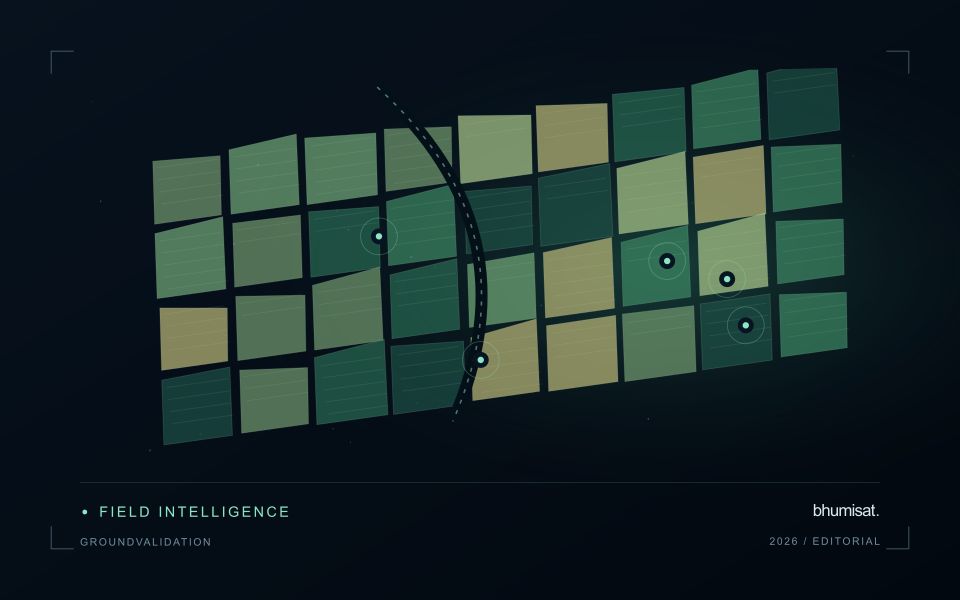
Maintain parcel or management boundaries where they are relevant and review whether the image resolution can separate the features of interest. Small geometric offsets can alter a comparison along narrow roads or building edges. Seasonal crop changes, temporary clearing and construction activity may produce different explanations for similar spectral patterns. Retain the acquisition dates and quality context, particularly when the available observations leave uncertainty about when a transition occurred.
Field validation should identify the current surface and its documented use as separate attributes. Record the location, date and spatial extent represented by each observation, and include unchanged parcels as well as obvious transitions. A useful product provides an auditable inventory of observed changes and their uncertainty. More specific conclusions about development status, ownership or future use require appropriate external records rather than inference from image appearance alone.
Identify what changes between domains
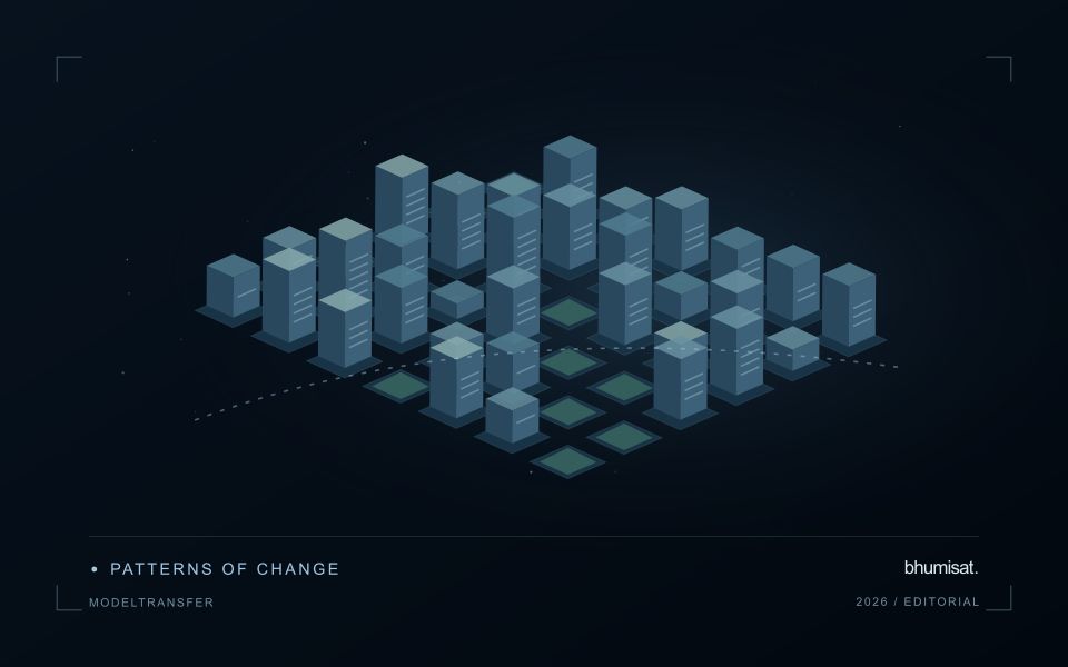
A model trained on one region or season learns relationships present in its development data. Applying it elsewhere assumes those relationships remain useful. New crop varieties, forest types, soil colours, management practices, illumination, or sensor characteristics can violate that assumption. Define the intended transfer explicitly: a new district, another year, another sensor, or a different class distribution. Each change creates a different test. A model that transfers across nearby fields has not thereby demonstrated reliable performance across climates or observation systems.
Keep the measurement pipeline consistent before attributing differences to the model. Reflectance scaling, band order, cloud masking, spatial resolution, composite windows, and missing value handling can all change predictions. Sensors with similarly named bands may have different spectral responses. Harmonization can reduce some differences but does not establish equivalence for every target. Examine predictor distributions, missing data rates, and examples from the new setting. Flag inputs outside the conditions represented during training so that extrapolation remains visible.
Test the destination, then adapt carefully
Design evaluation splits around the intended deployment. Hold out geographic regions to test spatial transfer and later years to test temporal transfer, keeping neighboring samples or repeated observations of the same site together when needed. Report performance for meaningful destination groups rather than only a pooled score. Class prevalence affects some metrics, so interpret changes alongside the underlying confusion matrix or residual distributions. A random pixel split can look excellent while providing little evidence about performance in an unseen region.
If local labels are available, reserve a destination assessment set before fine tuning or recalibration. Use the remaining observations to compare straightforward baselines with more complex adaptation methods. Check whether improvement comes from genuine transfer or simply from adding representative local data. Retain an option to withhold predictions when input quality or novelty makes them unreliable. Document the training domain, destination evidence, preprocessing versions, and conditions where use is unsupported. Continue monitoring once new observations arrive, since seasonal and environmental shifts can emerge after an initial evaluation. Transferability is a measured property of a particular model, workflow, target, and destination; it should not be inferred from architecture name or strong performance on the original test set.
Locate the uncertainty that matters to the decision
An uncertainty budget is a practical description of where a result could become unreliable. Begin with the observation chain: acquisition, calibration, geographic matching, reference measurements, feature calculation, modelling, and delivery. Identify the assumptions at each stage and ask which could materially change the interpretation. The purpose is not to assign a precise number to every limitation. It is to locate the sources that deserve attention for the intended decision.
Separate limitations that can be measured from those that currently require a qualitative description. Repeated measurements may help characterise variability, while comparisons with independent references can reveal systematic differences. Some uncertainties interact, so combining individual error estimates without examining their relationships can produce a misleading impression of precision. Keep the method of assessment visible and avoid treating an unexamined assumption as though it were a negligible contribution.
Use the budget to prioritise further work. The largest visible source of variation is not always the one whose reduction would most improve the decision. Consider which additional observation, test, or contextual record would change confidence in an actionable way. Revisit the budget when the application, observation source, or deployment conditions change. This turns uncertainty analysis into a guide for improving the workflow rather than a qualification added only after the result has been delivered.
Design an evaluation that reflects deployment
A model evaluation should resemble the conditions in which the model will be used. Start by identifying which relationships the development data share: nearby locations, repeated observations of the same unit, common collection teams, or measurements from a single period. These relationships can make records less independent than they appear. An evaluation that ignores them may test the ability to recognise familiar conditions rather than the ability to operate in a new setting.
Choose a split strategy that matches the intended transfer. Holding out locations, seasons, operational units, or acquisition conditions can answer different questions. Document which question each split is designed to address, and keep the held-out evidence separate while selecting features and tuning the method. Repeatedly inspecting the same evaluation set to improve a model gradually makes that set part of development, even if it retains its original label.
Report results at a scale that is meaningful to the user. A strong average can hide poor performance for important subgroups or unusual conditions. Examine error patterns and retain examples of both successful and unsuccessful predictions. Where the evidence covers only a limited range of conditions, describe that range explicitly. The evaluation then becomes a practical guide to suitable use, further testing, and the collection of additional reference observations.
Bring the evidence back to the decision
A strong interpretation states what was observed, which explanations remain plausible, and what additional evidence would help distinguish them. Avoid presenting a convenient label as a confirmed cause when the measurements support only a broader pattern. Connect the proposed next step to the significance of the decision and the confidence available. This creates an interpretation that a field team, analyst, or project partner can examine, challenge, and improve as further observations become available.
Sources & further reading
Explore the bhumisat spacecraft concept and our vision towards 2030, or return to the journal.