Comparisons through time are valuable only when the observations are sufficiently comparable for the question being asked. A difference between dates can reflect real change, a normal stage in a seasonal cycle, or a difference in how the surface was observed. This perspective examines the reference period, the timing of acquisitions, and the contextual records needed to interpret a sequence. It encourages the use of appropriate baselines rather than treating every previous observation as an equivalent benchmark. The objective is to identify changes that remain meaningful after normal variation and measurement conditions are considered.
This working guide considers mixed pixels and field boundary effects in open-field tomato production. The immediate decision is to select tomato rows for crop review. Useful reference evidence includes transplanting dates, canopy observations and field management notes. The case is an illustrative planning context, with assumptions to check against the actual sensor, landscape and project requirements.
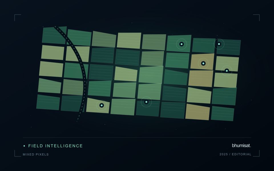
A pixel can represent several surface components
A satellite pixel represents an observation over a ground area, influenced by the instrument's spatial response and the scene within it. That area may contain several materials, such as crop canopy, soil, shade, water or a road. A mixed response is therefore common, especially near boundaries and in fragmented landscapes. It should not be treated automatically as a processing defect. The analytical question is whether the mixture supports the intended interpretation and whether a model trained under one mixture remains applicable under another.
Field geometry affects the number and character of observations available. A compact large field can contain many interior pixels, while a narrow or irregular field may consist mostly of boundary observations. Simply counting pixels does not establish how much independent information a dataset provides. Resampling onto a finer grid also does not remove the original mixing. Before selecting a monitoring product, examine the relationship between field dimensions, relevant landscape features and the measured spatial characteristics of the imagery that will support the service.
Choose a reporting unit that the data can support
Boundary exclusions can help investigate sensitivity to neighbouring surfaces, but they need a consistent rule and a clear purpose. Excluding a fixed distance may remove much of a small field while leaving a substantial interior in a larger one. Report the area retained and consider whether the remaining pixels represent the management unit fairly. Compare full-field and interior summaries during method development. A large difference can reveal a boundary or mixture problem that deserves attention before an alert is presented as a crop condition.
Validation should use observations collected at a scale compatible with the satellite interpretation. A measurement from a single plant or a small isolated plot may not describe the larger mixed area observed from orbit. Document the spatial support of both datasets and consider stratified sampling across relevant components. If the application requires information finer than the data can support, seek a suitable complementary source or change the question. Recognising mixed pixels helps an analyst design a credible product instead of assigning field-level precision to an observation that contains several different surfaces.
The setting: Open-field tomato production
Open-field tomato production can involve short management cycles, staggered planting and repeated operations within neighbouring parcels. The field calendar is therefore central to interpreting a satellite observation. Newly transplanted plants, established rows and areas nearing the end of production can show different responses for ordinary reasons. Record the planted area and the relevant management unit carefully, particularly where a commercial holding contains several crops or planting stages at the same time.
The image footprint may mix plants with soil, mulch, access routes and irrigation infrastructure. Determine whether the spatial resolution supports the intended row-level interpretation or whether a broader field summary is more appropriate. Examine the quality and age of observations before proposing a management use that depends on rapid response. A monitoring workflow should communicate when cloud gaps or the acquisition schedule leave insufficient current evidence for that decision.
Validation should document crop stage, canopy continuity, recent operations and the area represented by each sample. Field staff may use a mapped anomaly to choose an inspection location, but the subsequent diagnosis requires suitable observations and expertise. If production or quality is the target, collect reference information for those outcomes rather than assuming that greener vegetation implies more marketable fruit. The evaluation should measure whether the product improves a defined scouting or management process.
Define a representative reference sample
A reference sample should represent the situations in which a method will be used. Begin by defining the target population: locations, time periods, management conditions, surface types, or instrument states that belong within the intended application. A collection of convenient observations may be valuable for exploration, but it does not automatically support conclusions about that wider population. Make the scope of the sample visible before calculating a summary of performance.
Consider a stratified design when important conditions are unevenly represented. Relevant strata might include different landscape types, developmental stages, observation quality levels, or ranges of the variable being estimated. Choose sample locations within those groups using a documented rule, and retain the information needed to understand their selection. Where access restrictions affect the sample, record the excluded conditions so that the limits of the resulting evaluation remain clear.
Keep development and evaluation evidence separate where the purpose of the study requires an independent test. Nearby observations or repeated measurements can share information, so a random split of individual records may overstate independence. A split organised by location, period, or operational unit can provide a more demanding comparison. The appropriate design follows the intended deployment, the structure of the observations, and the errors that matter to the user.
Maintain the geographic units of analysis
Many observation services summarise measurements within a field, management block, catchment, forest unit, or other mapped boundary. The meaning of that summary depends on whether the boundary accurately represents the unit being discussed. Start with a clear source for the geometry and record its date, coordinate reference, and intended use. A boundary drawn for visual orientation may require additional checking before it becomes a measurement unit.
Inspect overlaps, gaps, narrow fragments, and features that may have changed since mapping. A geometrically valid polygon can still describe an outdated operational unit. Ask the responsible team how divisions, mergers, new infrastructure, and management changes are recorded. Where pixels or reference measurements cross a boundary, define how they are assigned or excluded so that results remain comparable between analysts and processing runs.
Version the boundaries alongside the observations. If a unit changes, preserve a relationship between the previous and revised geometry rather than replacing the history without explanation. Comparisons through time should identify whether they use a constant spatial unit or the operational units valid at each date. This makes it easier to distinguish a change in the measured surface from a change introduced by the geography used to summarise it.
Bring the evidence back to the decision
A useful comparison preserves the dates, quality conditions, and contextual assumptions behind its baseline. Review unusual results against the actual observation sequence rather than relying entirely on a summary statistic. Where seasonal timing is important, describe how comparable stages were identified. The resulting analysis should help users distinguish an informative change from an expected cycle or an observation artefact, while making gaps and remaining uncertainty visible enough to guide further investigation.
Sources & further reading
Explore the bhumisat spacecraft concept and our vision towards 2030, or return to the journal.