Every observation and interpretation contains uncertainty, but the sources and consequences of that uncertainty differ between applications. Some arise from acquisition conditions, others from reference measurements, processing choices, or the transfer of a model to a new setting. This perspective examines how those sources affect the decision a user is considering. It encourages teams to describe uncertainty in a form that can influence action, rather than adding a generic qualification at the end of a report. The objective is to support proportionate decisions while keeping the limits of the available evidence understandable.
This working guide considers harmonising satellite observation time series in soybean production fields. The immediate decision is to direct scouting to unusual field zones. Useful reference evidence includes planting dates, canopy closure and crop-stage observations. The case is an illustrative planning context, with assumptions to check against the actual sensor, landscape and project requirements.
More observations require a common measurement definition
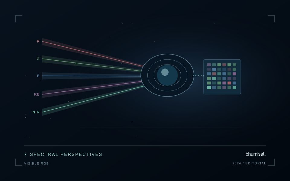
Combining observations from different satellites can increase the information available through time, but the resulting series needs a common analytical definition. Instruments may differ in spectral response, spatial sampling, viewing geometry and processing history. Two bands with similar names are not necessarily equivalent measurements. Harmonisation addresses selected differences so that observations can be used together more consistently. It should be understood as a documented processing approach with remaining limitations, rather than a guarantee that every value from every sensor is interchangeable.
A suitable workflow begins with the variables that need to be compared. Identify the input products, their physical meaning and the transformations already applied. A common grid helps organise observations spatially, while atmospheric correction, geometry normalisation and spectral adjustments may address other differences. These operations have distinct purposes. Applying only one of them should not be described as complete harmonisation. Retain sensor identity and acquisition metadata even when the user sees one combined series, because those attributes remain valuable for diagnosing an apparent discontinuity.
Validate continuity before interpreting a longer record
Test continuity using overlapping or otherwise comparable observations and independent evidence where available. Inspect several surface types and canopy conditions rather than evaluating only one convenient landscape. A consistent average relationship can still hide a meaningful difference for a particular crop or season. Examine how the combined record affects the final product, including index thresholds, fitted timing metrics and change alerts. The relevant question is whether the remaining differences are acceptable for that application, not merely whether the images appear similar on a map.
A longer record also requires a stable policy for quality screening and updates. Changes in input collections, calibration or processing versions can affect historical outputs. Version the workflow and preserve enough information to reproduce earlier results when necessary. When a series crosses a known processing change, evaluate the transition explicitly. A harmonised dataset can provide a strong foundation for monitoring, but field context and validation still determine the usefulness of its interpretation. Maintaining traceability allows additional observations to improve coverage without concealing their origins or implying a precision that has not been demonstrated.
The setting: Soybean production fields
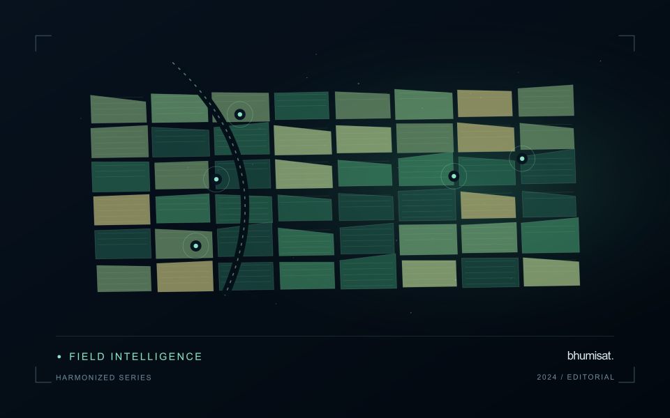
Soybean imagery can show substantial variation as fields progress from exposed soil to closed canopy and eventually to maturity. Planting date, stand arrangement, variety and management can shift that progression. Use these factors to define comparison groups before labelling a field unusual. The boundary dataset should distinguish the planted area from tracks, drainage features and other surfaces that can contribute a large share of the measurement in small or irregular fields.
A practical analytical sequence combines quality-screened imagery with the field calendar and relevant management notes. Review whether an apparent difference persists across usable observations and whether it follows a plausible spatial pattern within the field. An index response can be affected by background soil, weeds, residue or illumination as well as the crop. These possibilities should guide the investigation rather than being collapsed into an automatic claim about plant nutrition or disease.
A field team can test whether the mapped zones correspond to different crop stages or other observable conditions. Collect samples across the range of mapped responses, and include typical areas to avoid evaluating only conspicuous anomalies. Where production estimates are proposed, match the spatial and temporal scale of the reference data to the prediction. A field-average yield record cannot directly validate every small pixel-level variation shown on an attractive map.
Use observation labels with consistent meanings
A reference label should describe an observation that another person could recognise or reproduce. Broad terms such as good, damaged, or unusual can conceal substantial differences between collection teams. Begin by defining the feature or condition being recorded, the observation unit, and the evidence needed to assign a label. Where possible, distinguish a direct measurement from an interpretation made by the observer.
Provide a short collection guide with examples, boundary cases, and a way to record uncertainty. Train observers using shared cases before relying on independently collected labels. If two observers disagree, preserve the disagreement long enough to understand its cause. It may reveal an unclear definition, a genuinely ambiguous condition, a difference in observation scale, or a problem in matching the reference record to the remote measurement.
Retain the context that makes the label interpretable. Location, time, collection method, observer role, and relevant surface conditions can be essential for later review. Changes to the label scheme should be documented and related to earlier versions where a defensible correspondence exists. Consistent labels do not eliminate uncertainty, but they make it possible to investigate disagreement, evaluate analytical methods, and identify where better definitions or additional measurements would improve the evidence.
Maintain the geographic units of analysis
Many observation services summarise measurements within a field, management block, catchment, forest unit, or other mapped boundary. The meaning of that summary depends on whether the boundary accurately represents the unit being discussed. Start with a clear source for the geometry and record its date, coordinate reference, and intended use. A boundary drawn for visual orientation may require additional checking before it becomes a measurement unit.
Inspect overlaps, gaps, narrow fragments, and features that may have changed since mapping. A geometrically valid polygon can still describe an outdated operational unit. Ask the responsible team how divisions, mergers, new infrastructure, and management changes are recorded. Where pixels or reference measurements cross a boundary, define how they are assigned or excluded so that results remain comparable between analysts and processing runs.
Version the boundaries alongside the observations. If a unit changes, preserve a relationship between the previous and revised geometry rather than replacing the history without explanation. Comparisons through time should identify whether they use a constant spatial unit or the operational units valid at each date. This makes it easier to distinguish a change in the measured surface from a change introduced by the geography used to summarise it.
Bring the evidence back to the decision
Useful uncertainty communication identifies the limitation, explains how it could affect the result, and connects it to a practical response. Some decisions can proceed with a qualified estimate; others require another observation or an independent check. Preserve uncertainty information through processing and delivery so that it is available at the point of use. This makes the analysis more accountable and gives the team a clearer basis for deciding which additional evidence would most improve the outcome.
Sources & further reading
Explore the bhumisat spacecraft concept and our vision towards 2030, or return to the journal.