Remote observations show patterns, while practical decisions depend on explaining what those patterns could mean. Interpretation therefore requires more than locating a high or low value on a map. A useful analysis considers the timing of the observation, the physical processes that influence the measurement, and the information available from complementary sources. This perspective separates an observed signal from a proposed explanation and from an action recommended to a user. Keeping those stages distinct makes it easier to investigate alternative causes, communicate ambiguity, and choose a proportionate next step.
This working guide considers harmonising satellite observation time series across estuarine mixing zones. The immediate decision is to plan sampling across estuarine gradients. Useful reference evidence includes tidal stage, sample timing and water-variable measurements. The case is an illustrative planning context, with assumptions to check against the actual sensor, landscape and project requirements.
The setting: Estuarine mixing zones
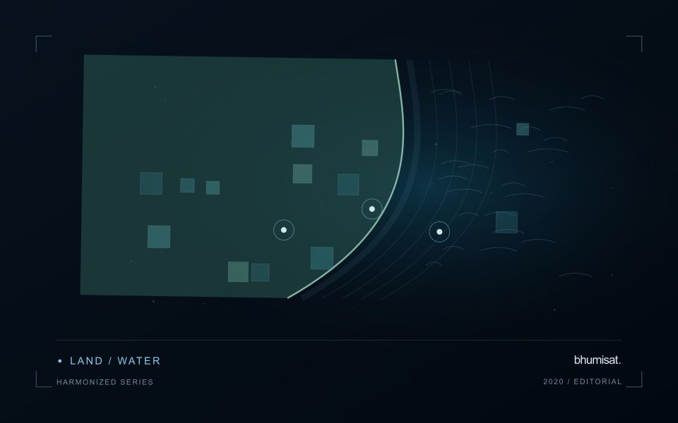
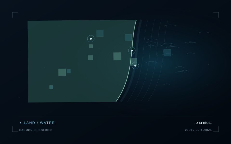
An estuary connects river inflow, coastal water, tidal conditions and complex shorelines. The resulting image pattern may change even when a monitoring team has not altered its methods. A useful design begins with a specific question, such as mapping visible water or investigating a persistent spectral gradient. It should not assume that one relationship describes every part of the estuary or that a single acquisition represents conditions throughout a tidal cycle.
Comparison units should account for channels, shallow margins and locations where land and water are mixed within an observation. Review cloud and atmospheric quality, surface reflection and geometric alignment before interpreting a difference between dates. Tidal and inflow context can help explain the setting but does not replace measurements of the target variable. Preserve the acquisition times and valid areas so that a mapped feature can be evaluated against the conditions under which it was observed.
A validation plan should represent different water types and spatial positions across the mixing zone. Collect the timing and location of samples consistently, and consider whether conditions changed between sampling and acquisition. A spectral boundary may help organise an investigation without proving a particular source or ecological consequence. More specific interpretations require evidence designed for those claims, while an auditable record of observed patterns and sampling priorities can already improve the structure of a monitoring programme.
More observations require a common measurement definition
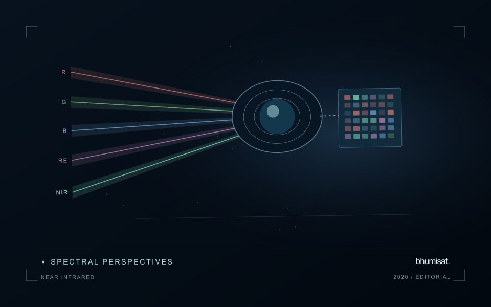
Combining observations from different satellites can increase the information available through time, but the resulting series needs a common analytical definition. Instruments may differ in spectral response, spatial sampling, viewing geometry and processing history. Two bands with similar names are not necessarily equivalent measurements. Harmonisation addresses selected differences so that observations can be used together more consistently. It should be understood as a documented processing approach with remaining limitations, rather than a guarantee that every value from every sensor is interchangeable.
A suitable workflow begins with the variables that need to be compared. Identify the input products, their physical meaning and the transformations already applied. A common grid helps organise observations spatially, while atmospheric correction, geometry normalisation and spectral adjustments may address other differences. These operations have distinct purposes. Applying only one of them should not be described as complete harmonisation. Retain sensor identity and acquisition metadata even when the user sees one combined series, because those attributes remain valuable for diagnosing an apparent discontinuity.
Validate continuity before interpreting a longer record
Test continuity using overlapping or otherwise comparable observations and independent evidence where available. Inspect several surface types and canopy conditions rather than evaluating only one convenient landscape. A consistent average relationship can still hide a meaningful difference for a particular crop or season. Examine how the combined record affects the final product, including index thresholds, fitted timing metrics and change alerts. The relevant question is whether the remaining differences are acceptable for that application, not merely whether the images appear similar on a map.
A longer record also requires a stable policy for quality screening and updates. Changes in input collections, calibration or processing versions can affect historical outputs. Version the workflow and preserve enough information to reproduce earlier results when necessary. When a series crosses a known processing change, evaluate the transition explicitly. A harmonised dataset can provide a strong foundation for monitoring, but field context and validation still determine the usefulness of its interpretation. Maintaining traceability allows additional observations to improve coverage without concealing their origins or implying a precision that has not been demonstrated.
Design an evaluation that reflects deployment
A model evaluation should resemble the conditions in which the model will be used. Start by identifying which relationships the development data share: nearby locations, repeated observations of the same unit, common collection teams, or measurements from a single period. These relationships can make records less independent than they appear. An evaluation that ignores them may test the ability to recognise familiar conditions rather than the ability to operate in a new setting.
Choose a split strategy that matches the intended transfer. Holding out locations, seasons, operational units, or acquisition conditions can answer different questions. Document which question each split is designed to address, and keep the held-out evidence separate while selecting features and tuning the method. Repeatedly inspecting the same evaluation set to improve a model gradually makes that set part of development, even if it retains its original label.
Report results at a scale that is meaningful to the user. A strong average can hide poor performance for important subgroups or unusual conditions. Examine error patterns and retain examples of both successful and unsuccessful predictions. Where the evidence covers only a limited range of conditions, describe that range explicitly. The evaluation then becomes a practical guide to suitable use, further testing, and the collection of additional reference observations.
Maintain the geographic units of analysis
Many observation services summarise measurements within a field, management block, catchment, forest unit, or other mapped boundary. The meaning of that summary depends on whether the boundary accurately represents the unit being discussed. Start with a clear source for the geometry and record its date, coordinate reference, and intended use. A boundary drawn for visual orientation may require additional checking before it becomes a measurement unit.
Inspect overlaps, gaps, narrow fragments, and features that may have changed since mapping. A geometrically valid polygon can still describe an outdated operational unit. Ask the responsible team how divisions, mergers, new infrastructure, and management changes are recorded. Where pixels or reference measurements cross a boundary, define how they are assigned or excluded so that results remain comparable between analysts and processing runs.
Version the boundaries alongside the observations. If a unit changes, preserve a relationship between the previous and revised geometry rather than replacing the history without explanation. Comparisons through time should identify whether they use a constant spatial unit or the operational units valid at each date. This makes it easier to distinguish a change in the measured surface from a change introduced by the geography used to summarise it.
Bring the evidence back to the decision
A strong interpretation states what was observed, which explanations remain plausible, and what additional evidence would help distinguish them. Avoid presenting a convenient label as a confirmed cause when the measurements support only a broader pattern. Connect the proposed next step to the significance of the decision and the confidence available. This creates an interpretation that a field team, analyst, or project partner can examine, challenge, and improve as further observations become available.
Sources & further reading
Explore the bhumisat spacecraft concept and our vision towards 2030, or return to the journal.