Comparisons through time are valuable only when the observations are sufficiently comparable for the question being asked. A difference between dates can reflect real change, a normal stage in a seasonal cycle, or a difference in how the surface was observed. This perspective examines the reference period, the timing of acquisitions, and the contextual records needed to interpret a sequence. It encourages the use of appropriate baselines rather than treating every previous observation as an equivalent benchmark. The objective is to identify changes that remain meaningful after normal variation and measurement conditions are considered.
This working guide considers harmonising satellite observation time series around aquaculture pond clusters. The immediate decision is to prioritise pond-cluster monitoring visits. Useful reference evidence includes pond boundaries, operation status and timed water measurements. The case is an illustrative planning context, with assumptions to check against the actual sensor, landscape and project requirements.
The setting: Aquaculture pond clusters
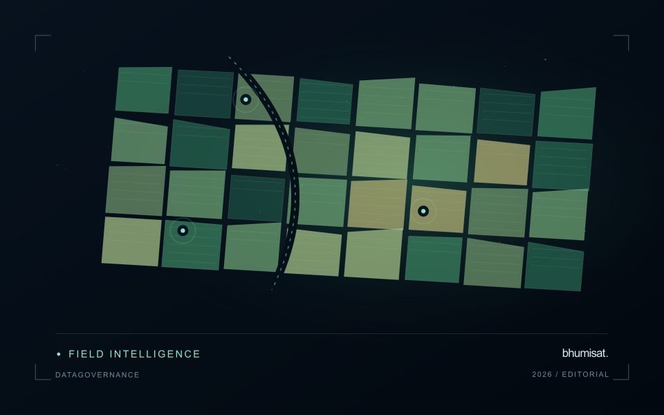
An aquaculture landscape contains ponds at different operating stages together with embankments, channels, roads and service areas. A satellite observation may support a pond inventory or a broader review of visible water patterns, but it should not be assumed to measure conditions within every individual production unit. Begin with boundaries and a record of pond status. Empty, recently filled and active ponds can have different appearances for ordinary operational reasons.
The size of a pond relative to the observation footprint determines how much embankment or neighbouring water contributes to a measurement. Review alignment and exclude unsuitable mixed areas where necessary. Surface reflections, cloud and atmospheric conditions can complicate optical comparison, while short-term management changes may occur between usable acquisitions. Retain observation dates and quality masks so that the image record does not imply continuous knowledge of rapidly changing pond conditions.
Validation should record the unit, collection time, operational context and the measurement method for any water variable being studied. A sample from one pond cannot automatically validate an adjacent pond or an entire cluster. A colour anomaly may help select a monitoring visit without establishing a particular biological condition or production outcome. More specific estimates require a demonstrated relationship with representative measurements, while inventory and inspection-priority products can be evaluated against the practical decisions they support.
More observations require a common measurement definition
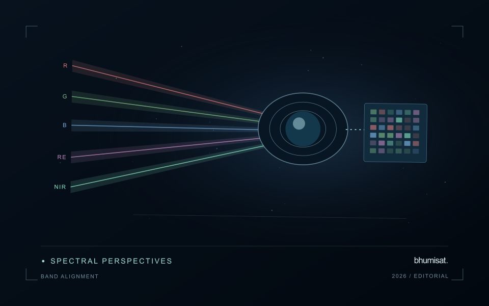
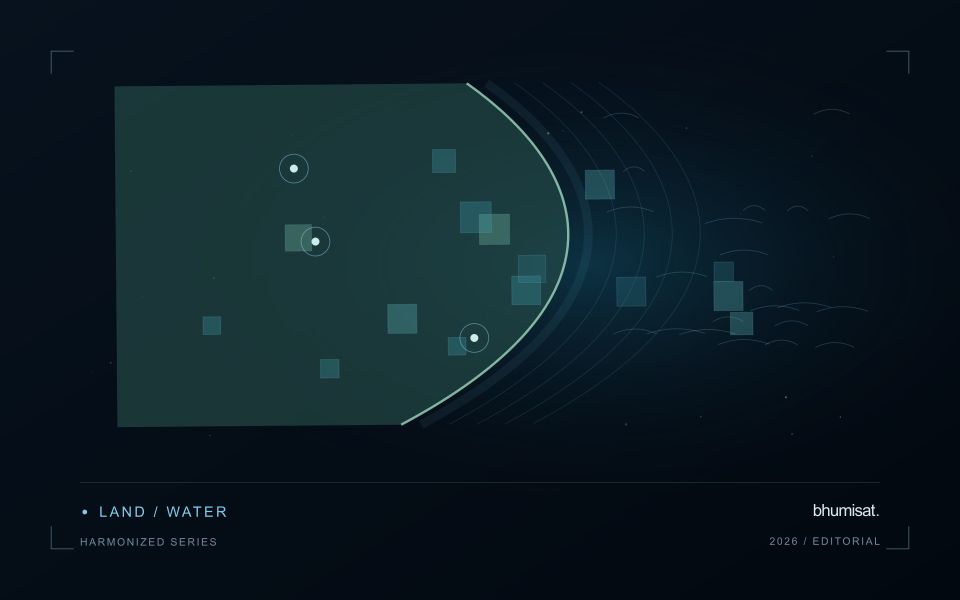
Combining observations from different satellites can increase the information available through time, but the resulting series needs a common analytical definition. Instruments may differ in spectral response, spatial sampling, viewing geometry and processing history. Two bands with similar names are not necessarily equivalent measurements. Harmonisation addresses selected differences so that observations can be used together more consistently. It should be understood as a documented processing approach with remaining limitations, rather than a guarantee that every value from every sensor is interchangeable.
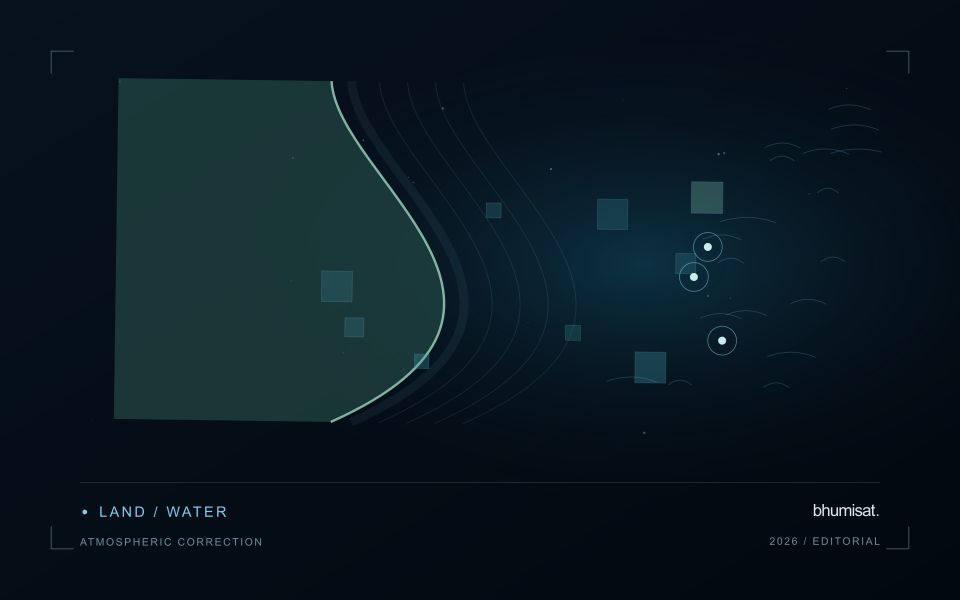
A suitable workflow begins with the variables that need to be compared. Identify the input products, their physical meaning and the transformations already applied. A common grid helps organise observations spatially, while atmospheric correction, geometry normalisation and spectral adjustments may address other differences. These operations have distinct purposes. Applying only one of them should not be described as complete harmonisation. Retain sensor identity and acquisition metadata even when the user sees one combined series, because those attributes remain valuable for diagnosing an apparent discontinuity.
Validate continuity before interpreting a longer record
Test continuity using overlapping or otherwise comparable observations and independent evidence where available. Inspect several surface types and canopy conditions rather than evaluating only one convenient landscape. A consistent average relationship can still hide a meaningful difference for a particular crop or season. Examine how the combined record affects the final product, including index thresholds, fitted timing metrics and change alerts. The relevant question is whether the remaining differences are acceptable for that application, not merely whether the images appear similar on a map.
A longer record also requires a stable policy for quality screening and updates. Changes in input collections, calibration or processing versions can affect historical outputs. Version the workflow and preserve enough information to reproduce earlier results when necessary. When a series crosses a known processing change, evaluate the transition explicitly. A harmonised dataset can provide a strong foundation for monitoring, but field context and validation still determine the usefulness of its interpretation. Maintaining traceability allows additional observations to improve coverage without concealing their origins or implying a precision that has not been demonstrated.
Represent gaps without inventing observations
A monitoring sequence often contains periods without a usable observation. The reason may be cloud, shadow, missing coverage, a failed transfer, or a quality condition that excludes the data. Begin by representing these states explicitly. A missing observation is different from a low measurement, an unchanged surface, or a confirmed absence of the feature being studied. The distinction should survive both the analysis and the presentation of the result.
Define when a temporal gap is acceptable for the intended decision. A workflow may continue using the latest qualified observation, request another source, or suspend an alert until sufficient evidence is available. Whichever response is selected, show the age of the supporting observation. If interpolation is used for a suitable analytical purpose, preserve the distinction between an estimated value and a directly observed measurement, together with the assumptions needed to interpret it.
Review how gaps affect the coverage of the final evaluation. Locations with frequent missing data may differ systematically from those with regular observations. A performance estimate based only on clear, complete records can therefore describe a narrower population than the service is expected to support. Report usable coverage alongside analytical results and use recurring gaps to guide acquisition planning, reference collection, and the selection of complementary observation methods.
Design an evaluation that reflects deployment
A model evaluation should resemble the conditions in which the model will be used. Start by identifying which relationships the development data share: nearby locations, repeated observations of the same unit, common collection teams, or measurements from a single period. These relationships can make records less independent than they appear. An evaluation that ignores them may test the ability to recognise familiar conditions rather than the ability to operate in a new setting.
Choose a split strategy that matches the intended transfer. Holding out locations, seasons, operational units, or acquisition conditions can answer different questions. Document which question each split is designed to address, and keep the held-out evidence separate while selecting features and tuning the method. Repeatedly inspecting the same evaluation set to improve a model gradually makes that set part of development, even if it retains its original label.
Report results at a scale that is meaningful to the user. A strong average can hide poor performance for important subgroups or unusual conditions. Examine error patterns and retain examples of both successful and unsuccessful predictions. Where the evidence covers only a limited range of conditions, describe that range explicitly. The evaluation then becomes a practical guide to suitable use, further testing, and the collection of additional reference observations.
Bring the evidence back to the decision
A useful comparison preserves the dates, quality conditions, and contextual assumptions behind its baseline. Review unusual results against the actual observation sequence rather than relying entirely on a summary statistic. Where seasonal timing is important, describe how comparable stages were identified. The resulting analysis should help users distinguish an informative change from an expected cycle or an observation artefact, while making gaps and remaining uncertainty visible enough to guide further investigation.
Sources & further reading
Explore the bhumisat spacecraft concept and our vision towards 2030, or return to the journal.