A workflow that succeeds on a small study area may encounter different constraints when the number of observations, locations, or users increases. Scaling requires attention to processing capacity, data organisation, reference coverage, and the effort needed to review results. This perspective looks beyond whether a calculation can run on a larger dataset. It asks whether the complete service can preserve its meaning, quality, and delivery commitments as its scope expands. The objective is a design that identifies bottlenecks early and increases throughput without silently weakening the evidence available to users.
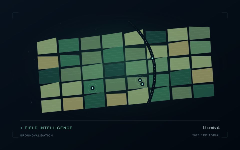
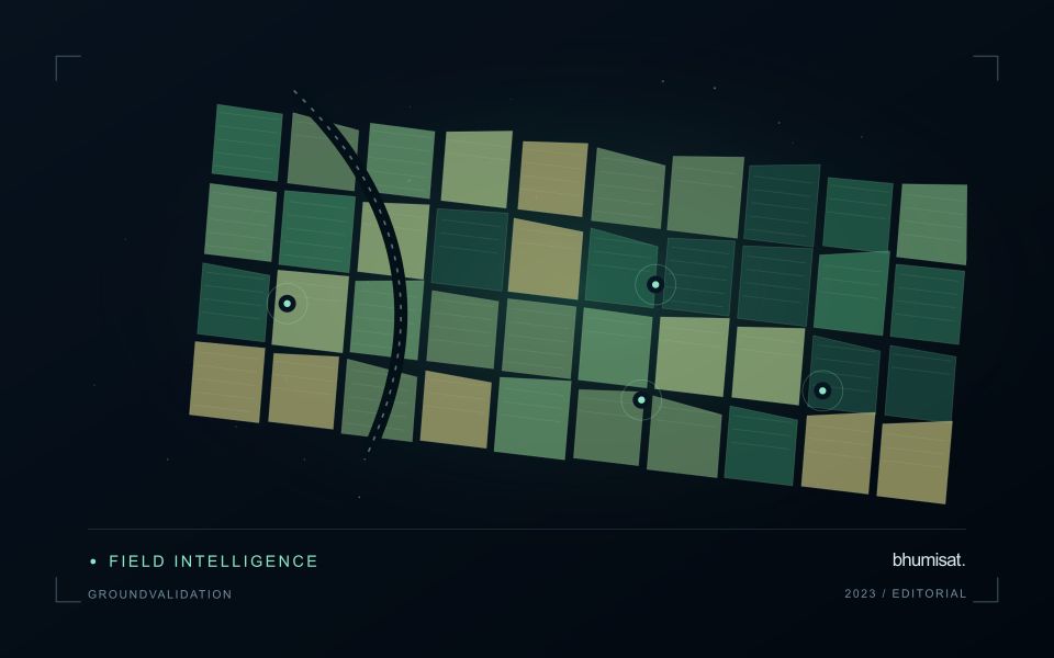
This working guide considers designing ground validation for satellite products in soybean production fields. The immediate decision is to direct scouting to unusual field zones. Useful reference evidence includes planting dates, canopy closure and crop-stage observations. The case is an illustrative planning context, with assumptions to check against the actual sensor, landscape and project requirements.
Start with the intended claim
Validation tests how well a product represents a defined quantity under specified conditions. It differs from calibration, which adjusts an instrument or model using reference information. Begin with the claim the product needs to support: class membership, surface reflectance, canopy height, water quality, or an area estimate. State the required spatial scale, time interval, and acceptable error. These choices determine the reference method and sample design. Collecting convenient field points first and deciding later what they prove usually leaves important conditions untested.
Reference measurements also contain uncertainty. Positioning error can place a sample in the wrong satellite pixel, a point instrument may not represent a heterogeneous footprint, and measurements made on different dates can describe real surface change. Record instrument calibration, sampling protocols, timestamps, coordinates, observation conditions, and uncertainty where available. For interpreted labels, retain the evidence used, class rules, and ambiguous cases. Agreement among interpreters is useful to examine, but agreement alone does not guarantee that the shared interpretation is correct.
Keep the assessment independent
Separate validation data from observations used to fit thresholds, train models, select features, or tune processing. If assessment sites repeatedly influence revisions, they have become development data and a fresh independent assessment is needed. Spatially clustered samples can make performance look stronger when neighboring training and test locations share conditions. Use a design that reflects the target population and report its limitations, including inaccessible areas or environmental conditions missing from the sample.
Choose metrics that match the product. For categorical maps, examine a confusion matrix and errors for individual classes, not just overall agreement. For continuous measurements, report bias and a suitable error measure alongside sample count and the range of reference values. Plot residuals against relevant conditions to expose failures hidden by an average. For area estimates, carry the probability sampling design through estimation and uncertainty calculations. Preserve rejected matchups and their reasons so that quality screening remains auditable. A useful validation report explains where the product works, where evidence is sparse, and which errors matter for the intended decision. Publishing reference protocols and assessment code makes later comparisons more credible and helps others reproduce the evaluation.
The setting: Soybean production fields
Soybean imagery can show substantial variation as fields progress from exposed soil to closed canopy and eventually to maturity. Planting date, stand arrangement, variety and management can shift that progression. Use these factors to define comparison groups before labelling a field unusual. The boundary dataset should distinguish the planted area from tracks, drainage features and other surfaces that can contribute a large share of the measurement in small or irregular fields.
A practical analytical sequence combines quality-screened imagery with the field calendar and relevant management notes. Review whether an apparent difference persists across usable observations and whether it follows a plausible spatial pattern within the field. An index response can be affected by background soil, weeds, residue or illumination as well as the crop. These possibilities should guide the investigation rather than being collapsed into an automatic claim about plant nutrition or disease.
A field team can test whether the mapped zones correspond to different crop stages or other observable conditions. Collect samples across the range of mapped responses, and include typical areas to avoid evaluating only conspicuous anomalies. Where production estimates are proposed, match the spatial and temporal scale of the reference data to the prediction. A field-average yield record cannot directly validate every small pixel-level variation shown on an attractive map.
Represent gaps without inventing observations
A monitoring sequence often contains periods without a usable observation. The reason may be cloud, shadow, missing coverage, a failed transfer, or a quality condition that excludes the data. Begin by representing these states explicitly. A missing observation is different from a low measurement, an unchanged surface, or a confirmed absence of the feature being studied. The distinction should survive both the analysis and the presentation of the result.
Define when a temporal gap is acceptable for the intended decision. A workflow may continue using the latest qualified observation, request another source, or suspend an alert until sufficient evidence is available. Whichever response is selected, show the age of the supporting observation. If interpolation is used for a suitable analytical purpose, preserve the distinction between an estimated value and a directly observed measurement, together with the assumptions needed to interpret it.
Review how gaps affect the coverage of the final evaluation. Locations with frequent missing data may differ systematically from those with regular observations. A performance estimate based only on clear, complete records can therefore describe a narrower population than the service is expected to support. Report usable coverage alongside analytical results and use recurring gaps to guide acquisition planning, reference collection, and the selection of complementary observation methods.
Use observation labels with consistent meanings
A reference label should describe an observation that another person could recognise or reproduce. Broad terms such as good, damaged, or unusual can conceal substantial differences between collection teams. Begin by defining the feature or condition being recorded, the observation unit, and the evidence needed to assign a label. Where possible, distinguish a direct measurement from an interpretation made by the observer.
Provide a short collection guide with examples, boundary cases, and a way to record uncertainty. Train observers using shared cases before relying on independently collected labels. If two observers disagree, preserve the disagreement long enough to understand its cause. It may reveal an unclear definition, a genuinely ambiguous condition, a difference in observation scale, or a problem in matching the reference record to the remote measurement.
Retain the context that makes the label interpretable. Location, time, collection method, observer role, and relevant surface conditions can be essential for later review. Changes to the label scheme should be documented and related to earlier versions where a defensible correspondence exists. Consistent labels do not eliminate uncertainty, but they make it possible to investigate disagreement, evaluate analytical methods, and identify where better definitions or additional measurements would improve the evidence.
Bring the evidence back to the decision
Expansion should be guided by measured workload, visible quality conditions, and an understanding of which tasks require expert attention. Test the workflow under representative data volumes before treating a successful demonstration as evidence of operational capacity. Preserve a route for investigating individual observations even when most processing is automated. A scalable service keeps its results traceable and useful as it grows, with clear choices about where to automate, where to review, and where to invest in additional evidence.
Sources & further reading
Explore the bhumisat spacecraft concept and our vision towards 2030, or return to the journal.