A workflow that succeeds on a small study area may encounter different constraints when the number of observations, locations, or users increases. Scaling requires attention to processing capacity, data organisation, reference coverage, and the effort needed to review results. This perspective looks beyond whether a calculation can run on a larger dataset. It asks whether the complete service can preserve its meaning, quality, and delivery commitments as its scope expands. The objective is a design that identifies bottlenecks early and increases throughput without silently weakening the evidence available to users.
This working guide considers geolocation accuracy for field-level monitoring in soybean production fields. The immediate decision is to direct scouting to unusual field zones. Useful reference evidence includes planting dates, canopy closure and crop-stage observations. The case is an illustrative planning context, with assumptions to check against the actual sensor, landscape and project requirements.
The setting: Soybean production fields
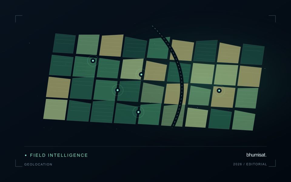
Soybean imagery can show substantial variation as fields progress from exposed soil to closed canopy and eventually to maturity. Planting date, stand arrangement, variety and management can shift that progression. Use these factors to define comparison groups before labelling a field unusual. The boundary dataset should distinguish the planted area from tracks, drainage features and other surfaces that can contribute a large share of the measurement in small or irregular fields.
A practical analytical sequence combines quality-screened imagery with the field calendar and relevant management notes. Review whether an apparent difference persists across usable observations and whether it follows a plausible spatial pattern within the field. An index response can be affected by background soil, weeds, residue or illumination as well as the crop. These possibilities should guide the investigation rather than being collapsed into an automatic claim about plant nutrition or disease.
A field team can test whether the mapped zones correspond to different crop stages or other observable conditions. Collect samples across the range of mapped responses, and include typical areas to avoid evaluating only conspicuous anomalies. Where production estimates are proposed, match the spatial and temporal scale of the reference data to the prediction. A field-average yield record cannot directly validate every small pixel-level variation shown on an attractive map.
Absolute location and relative alignment answer different questions
Geolocation describes where an observation is placed on Earth. For a field-level application, its quality affects which measurements are assigned to each management unit and whether an alert can be found during inspection. Absolute accuracy concerns the relationship with a suitable geographic reference. Relative alignment concerns the relationship between observations, such as images from different dates. A series can align well internally while still being displaced from a field boundary dataset. Both relationships should be considered when they matter to the intended decision.
The geographic reference includes more than a familiar coordinate system label. Map projection, datum, axis order, units and any relevant height reference can affect how data are combined. Field boundaries also have an origin and uncertainty of their own. A boundary drawn from an old image may not represent the current cultivated area, even if the satellite product is positioned correctly. Preserve the provenance of both the image and vector data, and distinguish a positional mismatch from a real change in land management.
Test accuracy at the management scale
Accuracy assessment needs independent, appropriate reference information distributed across the area of interest. Choosing only easy points can underrepresent difficult terrain or surface conditions. Define the feature being measured and check that it is identifiable at the image's spatial scale. Report the evaluation method and the distribution of residuals, rather than relying only on a single average error. A visual overlay is useful for finding issues, but it is not a substitute for an assessment designed around the accuracy claim being made.
The acceptable error depends on the task. A displacement that has little effect on a large plantation block may be consequential for a narrow field or a small validation plot. Evaluate how plausible location errors influence the derived statistic or operational instruction. Where necessary, revise the reporting unit, improve the reference data or obtain a complementary observation. The objective is not an impressive accuracy number in isolation. It is a defensible connection between the satellite measurement, the field record and the place where a person will use the result.
Check spatial alignment before comparison
A comparison between images, channels, maps, or field measurements assumes that the observations refer to the same locations at a suitable level of precision. Small alignment errors can become especially important near boundaries or narrow features. Before interpreting differences, inspect whether identifiable, stable features agree between the sources. A common coordinate reference is necessary for many workflows, but it does not by itself demonstrate accurate alignment.
Use control features that are appropriate for the observation scale and remain stable across the comparison period. Evaluate alignment in more than one part of the area, because a single location cannot reveal spatially varying distortion. Record the method used to estimate any correction and retain independent features for checking the corrected result. Where surfaces have genuinely changed, avoid using those changes as evidence of an alignment error.
Propagate the implications of remaining misalignment into the analysis. A workflow may exclude boundary pixels, summarise at a broader scale, or qualify interpretations for small features. The choice should follow the application rather than a preference for visually smooth output. Preserve both the original and corrected geographic references, and document resampling decisions so that future users can understand how measurements were moved onto a common spatial framework.
Represent gaps without inventing observations
A monitoring sequence often contains periods without a usable observation. The reason may be cloud, shadow, missing coverage, a failed transfer, or a quality condition that excludes the data. Begin by representing these states explicitly. A missing observation is different from a low measurement, an unchanged surface, or a confirmed absence of the feature being studied. The distinction should survive both the analysis and the presentation of the result.
Define when a temporal gap is acceptable for the intended decision. A workflow may continue using the latest qualified observation, request another source, or suspend an alert until sufficient evidence is available. Whichever response is selected, show the age of the supporting observation. If interpolation is used for a suitable analytical purpose, preserve the distinction between an estimated value and a directly observed measurement, together with the assumptions needed to interpret it.
Review how gaps affect the coverage of the final evaluation. Locations with frequent missing data may differ systematically from those with regular observations. A performance estimate based only on clear, complete records can therefore describe a narrower population than the service is expected to support. Report usable coverage alongside analytical results and use recurring gaps to guide acquisition planning, reference collection, and the selection of complementary observation methods.
Bring the evidence back to the decision
Expansion should be guided by measured workload, visible quality conditions, and an understanding of which tasks require expert attention. Test the workflow under representative data volumes before treating a successful demonstration as evidence of operational capacity. Preserve a route for investigating individual observations even when most processing is automated. A scalable service keeps its results traceable and useful as it grows, with clear choices about where to automate, where to review, and where to invest in additional evidence.
Sources & further reading
Explore the bhumisat spacecraft concept and our vision towards 2030, or return to the journal.