Comparisons through time are valuable only when the observations are sufficiently comparable for the question being asked. A difference between dates can reflect real change, a normal stage in a seasonal cycle, or a difference in how the surface was observed. This perspective examines the reference period, the timing of acquisitions, and the contextual records needed to interpret a sequence. It encourages the use of appropriate baselines rather than treating every previous observation as an equivalent benchmark. The objective is to identify changes that remain meaningful after normal variation and measurement conditions are considered.
This working guide considers geolocation accuracy for field-level monitoring in irrigated rice systems. The immediate decision is to identify fields needing irrigation review. Useful reference evidence includes field stage, inundation records and irrigation observations. The case is an illustrative planning context, with assumptions to check against the actual sensor, landscape and project requirements.
The setting: Irrigated rice systems
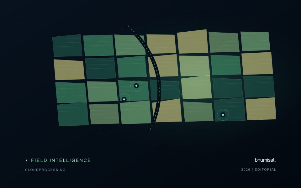
An irrigated rice landscape changes from preparation and inundation to crop establishment, canopy development and harvest. Water and vegetation contribute differently to the observed signal at these stages. A field should therefore be interpreted with its planting calendar and irrigation status, not only its latest colour on a map. Accurate paddy boundaries are valuable because bunds, channels, neighbouring fields and settlements can occupy a substantial share of a small observation unit.
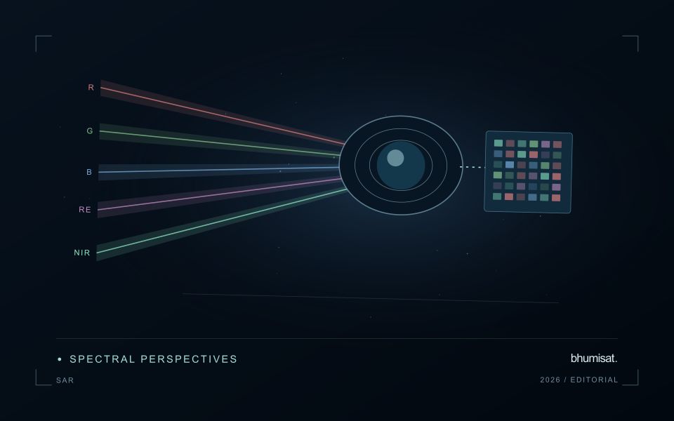
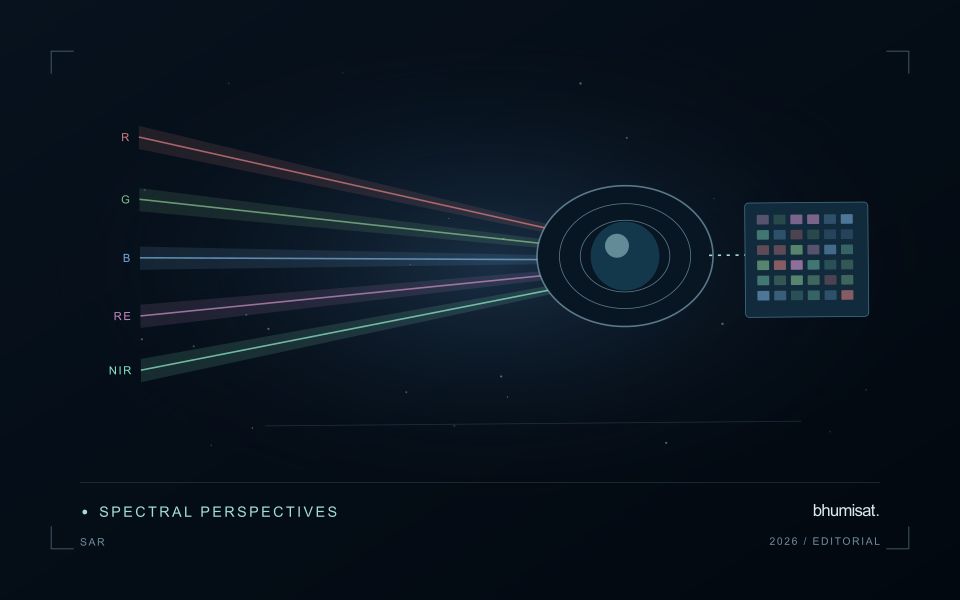
Organise the analysis around field-level sequences rather than a mosaic assembled from unrelated dates. In cloudy periods, identify gaps explicitly and consider which complementary observations are suitable for the question. Optical and radar measurements describe different physical properties, so their agreement or disagreement needs interpretation. An observation consistent with inundation is not by itself a complete account of irrigation delivery, field depth or the cause of a management problem.
A practical field visit records crop stage, water condition, planting method and the time of inspection. Irrigation managers may need a list of fields with unusual timing, while crop specialists may need areas of uneven development. These outputs require different validation records. Evaluate whether the information arrives early enough to support a decision, and retain observations of fields that were not flagged to understand missed events as well as false alerts.
Absolute location and relative alignment answer different questions
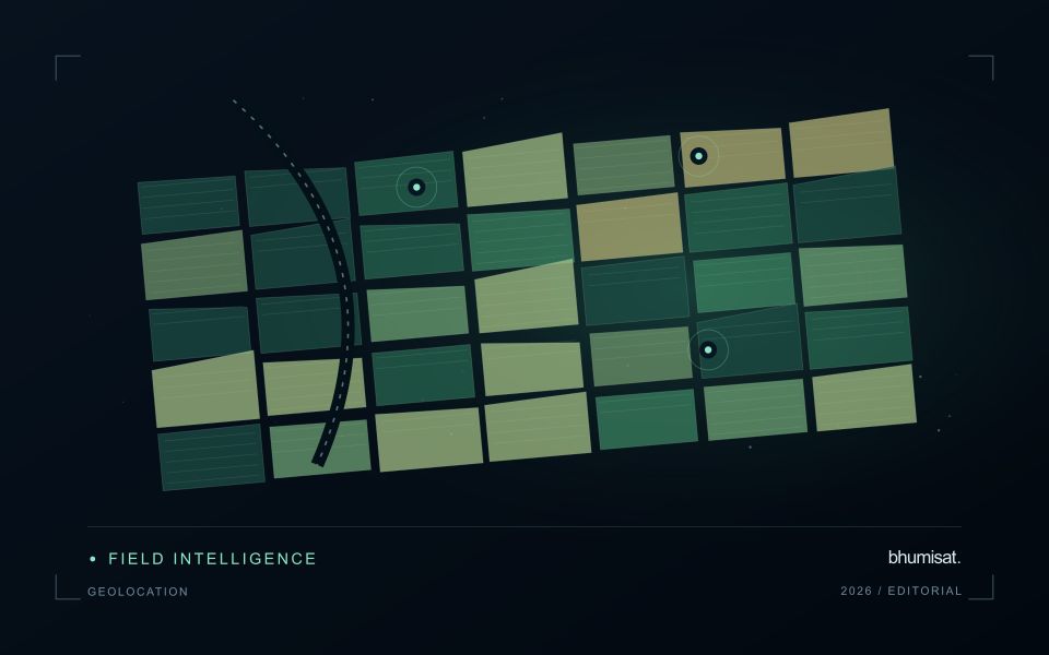
Geolocation describes where an observation is placed on Earth. For a field-level application, its quality affects which measurements are assigned to each management unit and whether an alert can be found during inspection. Absolute accuracy concerns the relationship with a suitable geographic reference. Relative alignment concerns the relationship between observations, such as images from different dates. A series can align well internally while still being displaced from a field boundary dataset. Both relationships should be considered when they matter to the intended decision.
The geographic reference includes more than a familiar coordinate system label. Map projection, datum, axis order, units and any relevant height reference can affect how data are combined. Field boundaries also have an origin and uncertainty of their own. A boundary drawn from an old image may not represent the current cultivated area, even if the satellite product is positioned correctly. Preserve the provenance of both the image and vector data, and distinguish a positional mismatch from a real change in land management.
Test accuracy at the management scale
Accuracy assessment needs independent, appropriate reference information distributed across the area of interest. Choosing only easy points can underrepresent difficult terrain or surface conditions. Define the feature being measured and check that it is identifiable at the image's spatial scale. Report the evaluation method and the distribution of residuals, rather than relying only on a single average error. A visual overlay is useful for finding issues, but it is not a substitute for an assessment designed around the accuracy claim being made.
The acceptable error depends on the task. A displacement that has little effect on a large plantation block may be consequential for a narrow field or a small validation plot. Evaluate how plausible location errors influence the derived statistic or operational instruction. Where necessary, revise the reporting unit, improve the reference data or obtain a complementary observation. The objective is not an impressive accuracy number in isolation. It is a defensible connection between the satellite measurement, the field record and the place where a person will use the result.
Locate the uncertainty that matters to the decision
An uncertainty budget is a practical description of where a result could become unreliable. Begin with the observation chain: acquisition, calibration, geographic matching, reference measurements, feature calculation, modelling, and delivery. Identify the assumptions at each stage and ask which could materially change the interpretation. The purpose is not to assign a precise number to every limitation. It is to locate the sources that deserve attention for the intended decision.
Separate limitations that can be measured from those that currently require a qualitative description. Repeated measurements may help characterise variability, while comparisons with independent references can reveal systematic differences. Some uncertainties interact, so combining individual error estimates without examining their relationships can produce a misleading impression of precision. Keep the method of assessment visible and avoid treating an unexamined assumption as though it were a negligible contribution.
Use the budget to prioritise further work. The largest visible source of variation is not always the one whose reduction would most improve the decision. Consider which additional observation, test, or contextual record would change confidence in an actionable way. Revisit the budget when the application, observation source, or deployment conditions change. This turns uncertainty analysis into a guide for improving the workflow rather than a qualification added only after the result has been delivered.
Design an evaluation that reflects deployment
A model evaluation should resemble the conditions in which the model will be used. Start by identifying which relationships the development data share: nearby locations, repeated observations of the same unit, common collection teams, or measurements from a single period. These relationships can make records less independent than they appear. An evaluation that ignores them may test the ability to recognise familiar conditions rather than the ability to operate in a new setting.
Choose a split strategy that matches the intended transfer. Holding out locations, seasons, operational units, or acquisition conditions can answer different questions. Document which question each split is designed to address, and keep the held-out evidence separate while selecting features and tuning the method. Repeatedly inspecting the same evaluation set to improve a model gradually makes that set part of development, even if it retains its original label.
Report results at a scale that is meaningful to the user. A strong average can hide poor performance for important subgroups or unusual conditions. Examine error patterns and retain examples of both successful and unsuccessful predictions. Where the evidence covers only a limited range of conditions, describe that range explicitly. The evaluation then becomes a practical guide to suitable use, further testing, and the collection of additional reference observations.
Bring the evidence back to the decision
A useful comparison preserves the dates, quality conditions, and contextual assumptions behind its baseline. Review unusual results against the actual observation sequence rather than relying entirely on a summary statistic. Where seasonal timing is important, describe how comparable stages were identified. The resulting analysis should help users distinguish an informative change from an expected cycle or an observation artefact, while making gaps and remaining uncertainty visible enough to guide further investigation.
Sources & further reading
Explore the bhumisat spacecraft concept and our vision towards 2030, or return to the journal.