A method that produces a plausible result has not automatically demonstrated that it works for its intended users. Validation requires a defined question, suitable reference evidence, and an evaluation design that reflects how the method will be used. This perspective examines which observations should be compared, how they should be sampled, and which errors matter in practice. It also considers the difference between evidence used to develop a method and evidence reserved for evaluating it. The objective is a test that can reveal weaknesses as well as confirm useful performance.
This working guide considers measuring forest cover without confusing canopy and land use on mountain forest slopes. The immediate decision is to select terrain-aware forest inspection sites. Useful reference evidence includes slope setting, canopy observations and reliable sample locations. The case is an illustrative planning context, with assumptions to check against the actual sensor, landscape and project requirements.
Define what the map measures
Forest cover is not a single self-evident quantity. One project may need the fraction of a pixel occupied by tree crowns; another may need a categorical forest mask based on canopy cover, height, and minimum area. A land use inventory may treat temporarily cleared forest differently from a map of visible tree cover. Write the definition before collecting labels, and identify how plantations, orchards, mangroves, sparse woodland, and urban trees will be handled. A consistent definition matters as much as a sophisticated classifier when comparing places or years.
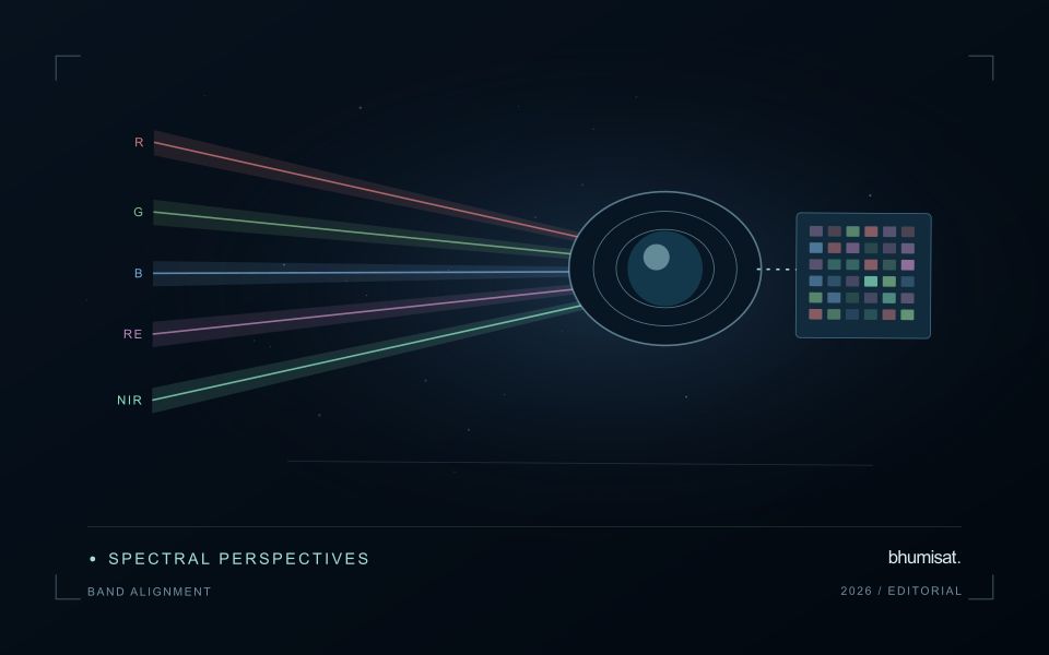
Optical observations provide information about foliage, moisture, and seasonal behavior, but similar vegetation types can have overlapping spectra. A green pixel does not establish tree height or distinguish a natural forest from a plantation. Time series can capture leaf emergence, dry season persistence, and disturbances that a single image misses. Radar adds sensitivity to vegetation structure and moisture, although relationships vary with wavelength, geometry, and forest conditions. Combining observations can improve discrimination when each input has a clear role and compatible spatial support.
Make estimates comparable and testable
Prepare a stable analysis grid, inspect geolocation, and apply consistent atmospheric and quality screening to optical inputs. Choose seasonal windows that suit the local ecology rather than assuming one calendar works everywhere. When clear observations are sparse, report the observation count and the age of the composite. Train with examples spanning forest types, canopy densities, topography, and confusing nonforest classes. Keep independent assessment locations separate from training areas, especially where neighboring pixels share the same stand.
Evaluate omission and commission errors for forest and relevant subclasses. A high overall accuracy can conceal poor performance in a rare forest type or along fragmented edges. For area reporting, use a probability sample and an estimator appropriate to its design rather than treating classified pixel counts as exact. Compare annual products with the same class definitions and processing assumptions. Abrupt canopy loss can indicate harvesting, fire, storms, or conversion, and the image alone may not identify the cause. Preserve that distinction in summaries, and accompany trend estimates with uncertainty and a description of what canopy recovery does and does not establish.
The setting: Mountain forest slopes
A mountain forest combines canopy complexity with strong changes in slope, aspect and illumination. Locations that contain similar vegetation may appear different because they are observed under different lighting conditions. A monitoring design should therefore consider terrain alongside its ecological question. Define whether it concerns cover change, disturbance or a particular forest parameter, and establish comparison units that do not confuse a shadowed slope with a different type or condition of forest.
Image selection and processing should retain the information needed to examine these effects. Cloud, terrain shadow and changing viewing geometry can limit the usable record in different ways. A detailed elevation model may help describe the setting, but its resolution and alignment also need consideration. Review boundary areas and narrow valleys carefully, where mixed surfaces or small spatial offsets can have a large influence on an apparent change.
Field observations should represent the range of terrain settings in which the monitoring result will be used. Convenient valley access points may not characterise conditions on upper slopes. Record the location, slope context, canopy structure and date of each sample, along with uncertainty in locating it. A successful interpretation should remain defensible across the relevant terrain range. Where that has not been demonstrated, present the observation as a terrain-aware inspection lead rather than a fully validated forest measurement.
Represent gaps without inventing observations
A monitoring sequence often contains periods without a usable observation. The reason may be cloud, shadow, missing coverage, a failed transfer, or a quality condition that excludes the data. Begin by representing these states explicitly. A missing observation is different from a low measurement, an unchanged surface, or a confirmed absence of the feature being studied. The distinction should survive both the analysis and the presentation of the result.
Define when a temporal gap is acceptable for the intended decision. A workflow may continue using the latest qualified observation, request another source, or suspend an alert until sufficient evidence is available. Whichever response is selected, show the age of the supporting observation. If interpolation is used for a suitable analytical purpose, preserve the distinction between an estimated value and a directly observed measurement, together with the assumptions needed to interpret it.
Review how gaps affect the coverage of the final evaluation. Locations with frequent missing data may differ systematically from those with regular observations. A performance estimate based only on clear, complete records can therefore describe a narrower population than the service is expected to support. Report usable coverage alongside analytical results and use recurring gaps to guide acquisition planning, reference collection, and the selection of complementary observation methods.
Define a representative reference sample
A reference sample should represent the situations in which a method will be used. Begin by defining the target population: locations, time periods, management conditions, surface types, or instrument states that belong within the intended application. A collection of convenient observations may be valuable for exploration, but it does not automatically support conclusions about that wider population. Make the scope of the sample visible before calculating a summary of performance.
Consider a stratified design when important conditions are unevenly represented. Relevant strata might include different landscape types, developmental stages, observation quality levels, or ranges of the variable being estimated. Choose sample locations within those groups using a documented rule, and retain the information needed to understand their selection. Where access restrictions affect the sample, record the excluded conditions so that the limits of the resulting evaluation remain clear.
Keep development and evaluation evidence separate where the purpose of the study requires an independent test. Nearby observations or repeated measurements can share information, so a random split of individual records may overstate independence. A split organised by location, period, or operational unit can provide a more demanding comparison. The appropriate design follows the intended deployment, the structure of the observations, and the errors that matter to the user.
Bring the evidence back to the decision
The validation record should explain the population represented by the test, the reference observations used, and the limitations of the comparison. Report meaningful errors alongside useful successes, and retain examples that challenge the method. Treat wider deployment as a new opportunity to evaluate transfer across relevant conditions. A well-designed validation programme gives users a defensible basis for deciding where the method is useful, where additional evidence is needed, and where another approach may be appropriate.
Sources & further reading
Explore the bhumisat spacecraft concept and our vision towards 2030, or return to the journal.