A workflow that succeeds on a small study area may encounter different constraints when the number of observations, locations, or users increases. Scaling requires attention to processing capacity, data organisation, reference coverage, and the effort needed to review results. This perspective looks beyond whether a calculation can run on a larger dataset. It asks whether the complete service can preserve its meaning, quality, and delivery commitments as its scope expands. The objective is a design that identifies bottlenecks early and increases throughput without silently weakening the evidence available to users.
This working guide considers mapping flood extent with optical and radar imagery in turbid coastal waters. The immediate decision is to identify coastal sampling priorities. Useful reference evidence includes water samples, surface conditions and acquisition-time context. The case is an illustrative planning context, with assumptions to check against the actual sensor, landscape and project requirements.
Read the water signal in context
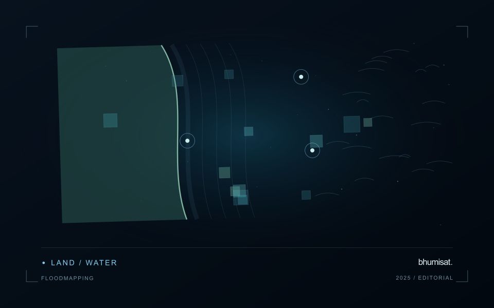
A flood extent map describes water visible at a particular observation time. It does not automatically describe maximum inundation, water depth, or the safety of a road. Begin by defining the event window, study boundary, permanent water baseline, and the smallest flooded area the analysis needs to represent. These decisions determine whether individual scenes, a time series, or several complementary sensors are appropriate. A satellite may pass after a short flood has already receded, so absence of mapped water is not evidence that flooding never occurred.
Optical imagery can separate open water from many surrounding surfaces because water strongly absorbs near infrared and shortwave infrared radiation. Clouds, cloud shadows, turbid water, floating vegetation, and dark roofs complicate that interpretation. Radar can observe through cloud and without sunlight, but its response depends on surface roughness, viewing geometry, polarization, and vegetation. Smooth open water often appears dark; wind can brighten it, while flooded vegetation can produce stronger returns. Neither a universal darkness threshold nor a single water index works reliably in every landscape.
Build and qualify an extent product
For optical analysis, use compatible reflectance products, inspect quality flags, and retain explicit masks for cloud and shadow. For radar, apply the corrections required by the selected product, account for terrain effects, and compare acquisitions with similar viewing geometry. A pre-event reference helps distinguish newly inundated land from reservoirs, wetlands, and persistent channels. Elevation and drainage information can expose implausible isolated detections, but a terrain rule should not silently remove real flooding behind an embankment.
Keep observed flood, permanent water, dry land, and unobserved areas as separate classes. Check results against independent reference observations collected close to acquisition time, including difficult boundaries and built environments. Document missed inundation and false alarms instead of reporting only a visually convincing example. Record acquisition timestamps, sensor and processing versions, thresholds, and validation limitations with the exported layer. When several dates are combined, identify the composite period clearly. An exposure overlay can then intersect the qualified extent with roads, settlements, or fields while preserving the distinction between observed water and inferred consequences.
The setting: Turbid coastal waters
Turbid coastal waters contain changing mixtures of suspended material, dissolved substances, biological components and surface reflections. Their image appearance may vary over short distances and between acquisitions. A monitoring design should identify which variable or pattern it aims to investigate rather than treating every colour difference as a direct water-quality measurement. Coastal geometry and the proximity of land also influence which parts of an image provide a defensible observation of water.
Review atmospheric conditions, cloud, shadow, sun glint and land adjacency before comparing spectral measurements. Shallow-bottom contributions can matter in some places, while deeper areas may present a different interpretation problem. A relationship developed for one water type should not be transferred automatically to another. Retain the valid observation mask and the dates supporting each map so that users can distinguish measured patterns from periods without suitable optical evidence.
Field validation should sample the range of conditions in which a model or interpretation rule will operate. Record collection time, location and the measurement method for the target variable, together with relevant surface conditions. Samples and imagery separated by a changing coastal event may not be comparable. A useful product can guide sampling or describe a consistent spectral pattern, with stronger numerical water-quality claims introduced only when their calibration and independent evaluation support the intended application.
Locate the uncertainty that matters to the decision
An uncertainty budget is a practical description of where a result could become unreliable. Begin with the observation chain: acquisition, calibration, geographic matching, reference measurements, feature calculation, modelling, and delivery. Identify the assumptions at each stage and ask which could materially change the interpretation. The purpose is not to assign a precise number to every limitation. It is to locate the sources that deserve attention for the intended decision.
Separate limitations that can be measured from those that currently require a qualitative description. Repeated measurements may help characterise variability, while comparisons with independent references can reveal systematic differences. Some uncertainties interact, so combining individual error estimates without examining their relationships can produce a misleading impression of precision. Keep the method of assessment visible and avoid treating an unexamined assumption as though it were a negligible contribution.
Use the budget to prioritise further work. The largest visible source of variation is not always the one whose reduction would most improve the decision. Consider which additional observation, test, or contextual record would change confidence in an actionable way. Revisit the budget when the application, observation source, or deployment conditions change. This turns uncertainty analysis into a guide for improving the workflow rather than a qualification added only after the result has been delivered.
Use observation labels with consistent meanings
A reference label should describe an observation that another person could recognise or reproduce. Broad terms such as good, damaged, or unusual can conceal substantial differences between collection teams. Begin by defining the feature or condition being recorded, the observation unit, and the evidence needed to assign a label. Where possible, distinguish a direct measurement from an interpretation made by the observer.
Provide a short collection guide with examples, boundary cases, and a way to record uncertainty. Train observers using shared cases before relying on independently collected labels. If two observers disagree, preserve the disagreement long enough to understand its cause. It may reveal an unclear definition, a genuinely ambiguous condition, a difference in observation scale, or a problem in matching the reference record to the remote measurement.
Retain the context that makes the label interpretable. Location, time, collection method, observer role, and relevant surface conditions can be essential for later review. Changes to the label scheme should be documented and related to earlier versions where a defensible correspondence exists. Consistent labels do not eliminate uncertainty, but they make it possible to investigate disagreement, evaluate analytical methods, and identify where better definitions or additional measurements would improve the evidence.
Bring the evidence back to the decision
Expansion should be guided by measured workload, visible quality conditions, and an understanding of which tasks require expert attention. Test the workflow under representative data volumes before treating a successful demonstration as evidence of operational capacity. Preserve a route for investigating individual observations even when most processing is automated. A scalable service keeps its results traceable and useful as it grows, with clear choices about where to automate, where to review, and where to invest in additional evidence.
Sources & further reading
Explore the bhumisat spacecraft concept and our vision towards 2030, or return to the journal.