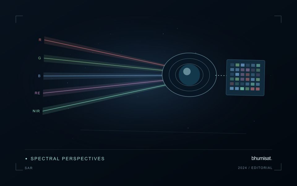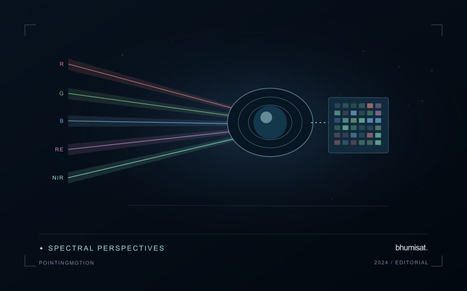
Comparisons through time are valuable only when the observations are sufficiently comparable for the question being asked. A difference between dates can reflect real change, a normal stage in a seasonal cycle, or a difference in how the surface was observed. This perspective examines the reference period, the timing of acquisitions, and the contextual records needed to interpret a sequence. It encourages the use of appropriate baselines rather than treating every previous observation as an equivalent benchmark. The objective is to identify changes that remain meaningful after normal variation and measurement conditions are considered.
This working guide considers mapping flood extent with optical and radar imagery across river floodplain areas. The immediate decision is to locate areas needing flood-impact review. Useful reference evidence includes dated water observations and representative field impact records. The case is an illustrative planning context, with assumptions to check against the actual sensor, landscape and project requirements.
Read the water signal in context
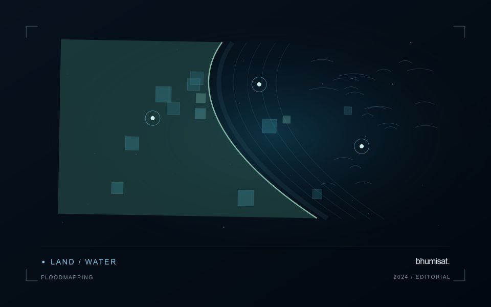
A flood extent map describes water visible at a particular observation time. It does not automatically describe maximum inundation, water depth, or the safety of a road. Begin by defining the event window, study boundary, permanent water baseline, and the smallest flooded area the analysis needs to represent. These decisions determine whether individual scenes, a time series, or several complementary sensors are appropriate. A satellite may pass after a short flood has already receded, so absence of mapped water is not evidence that flooding never occurred.
Optical imagery can separate open water from many surrounding surfaces because water strongly absorbs near infrared and shortwave infrared radiation. Clouds, cloud shadows, turbid water, floating vegetation, and dark roofs complicate that interpretation. Radar can observe through cloud and without sunlight, but its response depends on surface roughness, viewing geometry, polarization, and vegetation. Smooth open water often appears dark; wind can brighten it, while flooded vegetation can produce stronger returns. Neither a universal darkness threshold nor a single water index works reliably in every landscape.
Build and qualify an extent product
For optical analysis, use compatible reflectance products, inspect quality flags, and retain explicit masks for cloud and shadow. For radar, apply the corrections required by the selected product, account for terrain effects, and compare acquisitions with similar viewing geometry. A pre-event reference helps distinguish newly inundated land from reservoirs, wetlands, and persistent channels. Elevation and drainage information can expose implausible isolated detections, but a terrain rule should not silently remove real flooding behind an embankment.
Keep observed flood, permanent water, dry land, and unobserved areas as separate classes. Check results against independent reference observations collected close to acquisition time, including difficult boundaries and built environments. Document missed inundation and false alarms instead of reporting only a visually convincing example. Record acquisition timestamps, sensor and processing versions, thresholds, and validation limitations with the exported layer. When several dates are combined, identify the composite period clearly. An exposure overlay can then intersect the qualified extent with roads, settlements, or fields while preserving the distinction between observed water and inferred consequences.
The setting: River floodplain areas
A floodplain contains channels, low-lying fields, settlements, wetlands and surfaces that may be wet or dry under ordinary conditions. A flood-monitoring workflow should distinguish a new observation of water from the baseline distribution expected in that setting. Define the event period and the intended output, such as visible inundation extent or locations for field impact assessment. These products do not automatically establish water depth, damage or the cause of a particular local condition.
Cloud cover can limit optical observations during an event, while vegetation and structures may obscure water at the surface. Other observation types can contribute complementary evidence but require interpretation appropriate to their measurement physics. Compare suitable baseline and event acquisitions, check alignment and preserve the actual observation times. A map assembled from different dates should make those differences clear rather than implying that the whole floodplain was observed simultaneously.
Field validation should record when water or impacts were observed, the location and the area represented by each report. Conditions can change between an image acquisition and a visit, so apparent disagreement may reflect timing rather than a simple mapping error. Sample different land-cover settings and include places outside the mapped extent. A useful product communicates the evidence for observed inundation separately from estimates of damage or operational consequences that require further measurements.
Design an evaluation that reflects deployment
A model evaluation should resemble the conditions in which the model will be used. Start by identifying which relationships the development data share: nearby locations, repeated observations of the same unit, common collection teams, or measurements from a single period. These relationships can make records less independent than they appear. An evaluation that ignores them may test the ability to recognise familiar conditions rather than the ability to operate in a new setting.
Choose a split strategy that matches the intended transfer. Holding out locations, seasons, operational units, or acquisition conditions can answer different questions. Document which question each split is designed to address, and keep the held-out evidence separate while selecting features and tuning the method. Repeatedly inspecting the same evaluation set to improve a model gradually makes that set part of development, even if it retains its original label.
Report results at a scale that is meaningful to the user. A strong average can hide poor performance for important subgroups or unusual conditions. Examine error patterns and retain examples of both successful and unsuccessful predictions. Where the evidence covers only a limited range of conditions, describe that range explicitly. The evaluation then becomes a practical guide to suitable use, further testing, and the collection of additional reference observations.
Deliver quality flags that users can interpret
Quality information should describe the condition of an observation in terms that remain useful through the workflow. A single valid or invalid label may be sufficient for some calculations, but operational users often need to know why an observation was qualified. Distinguish acquisition limitations, processing failures, uncertain reference matches, and conditions that make interpretation ambiguous. These categories point towards different responses and should not be merged without a clear purpose.
Define a small, documented set of flags with stable meanings. Record whether a flag applies to a complete scene, a geographic unit, an individual measurement, or a derived result. A unit containing a mixture of qualified and unqualified observations may also require a coverage measure. Include the rule used to combine flags when summarising data so that a favourable average does not conceal a substantial fraction of unusable input.
Test the flags with the people receiving the product. Ask what they would do differently for each state and whether the terminology supports that choice. Keep the original flags available even if the interface presents a simpler summary. When flag definitions change, version the rules and review their effects on historical comparisons. Useful quality communication makes the condition of the evidence visible at the moment when a user decides how much confidence to place in the result.
Bring the evidence back to the decision
A useful comparison preserves the dates, quality conditions, and contextual assumptions behind its baseline. Review unusual results against the actual observation sequence rather than relying entirely on a summary statistic. Where seasonal timing is important, describe how comparable stages were identified. The resulting analysis should help users distinguish an informative change from an expected cycle or an observation artefact, while making gaps and remaining uncertainty visible enough to guide further investigation.
Sources & further reading
Explore the bhumisat spacecraft concept and our vision towards 2030, or return to the journal.