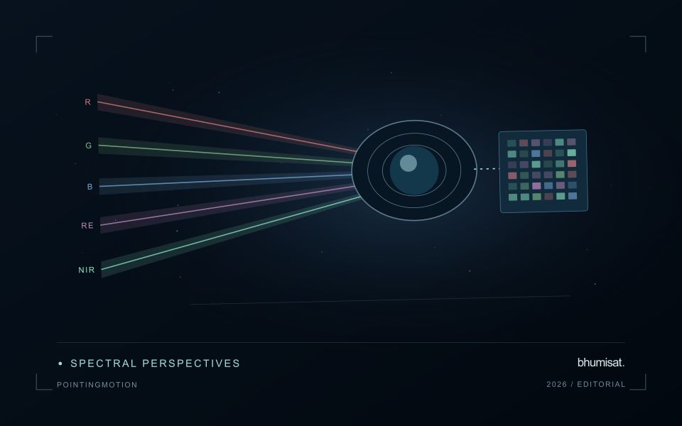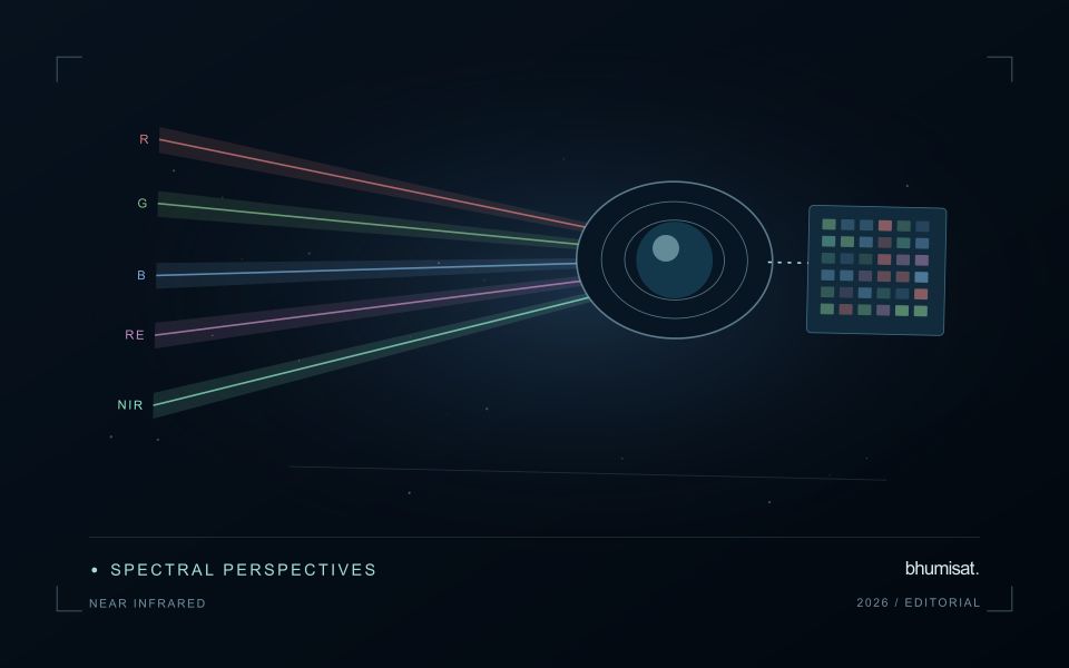
A workflow that succeeds on a small study area may encounter different constraints when the number of observations, locations, or users increases. Scaling requires attention to processing capacity, data organisation, reference coverage, and the effort needed to review results. This perspective looks beyond whether a calculation can run on a larger dataset. It asks whether the complete service can preserve its meaning, quality, and delivery commitments as its scope expands. The objective is a design that identifies bottlenecks early and increases throughput without silently weakening the evidence available to users.
This working guide considers choosing evi, savi and related indices across river floodplain areas. The immediate decision is to locate areas needing flood-impact review. Useful reference evidence includes dated water observations and representative field impact records. The case is an illustrative planning context, with assumptions to check against the actual sensor, landscape and project requirements.
Choose the index around the landscape
Vegetation indices emphasise selected relationships between spectral measurements. They are alternative views of the same observed surface, not independent diagnoses of a crop. EVI and SAVI were developed to address particular limitations encountered when interpreting vegetation signals, including background and canopy effects. Their usefulness depends on the data and landscape. A workflow should identify which limitation matters in its application before adding another index. Computing many indices without a clear comparison plan can increase complexity while leaving the original question unresolved.
SAVI introduces an adjustment intended to reduce sensitivity to soil brightness when vegetation cover is limited. The adjustment parameter should be chosen deliberately and retained in the processing record. EVI includes additional terms and commonly uses a blue band, making the quality of that measurement relevant to the result. Implementations must use the appropriate reflectance scaling and coefficient conventions. Applying a formula directly to stored integer values without considering offsets and scale factors can produce values that are mathematically calculable yet physically inconsistent.
Test whether the choice improves the decision
Compare candidate indices using the same quality-screened observations, field boundaries and independent evaluation sample. Otherwise a difference in performance might reflect a different set of pixels or dates rather than the index itself. Inspect sparse, intermediate and dense canopy conditions separately. Include soil exposure and recent management operations in the interpretation. A result that appears clearer on a colour map still needs to be tested against the variable of interest or the operational decision the service is expected to support.
The final choice should also account for maintenance and communication. An index that gives a modest improvement but depends on a less reliable band may require additional quality controls. Users should be told which observations were excluded and why a value is missing. Keep the selected method stable during an evaluation period, and version later changes so that historical comparisons remain interpretable. A concise set of well-understood indicators usually supports a stronger service than a long list of unexplained metrics that imply more certainty than the measurements justify.
The setting: River floodplain areas
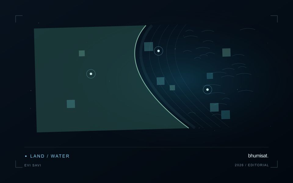
A floodplain contains channels, low-lying fields, settlements, wetlands and surfaces that may be wet or dry under ordinary conditions. A flood-monitoring workflow should distinguish a new observation of water from the baseline distribution expected in that setting. Define the event period and the intended output, such as visible inundation extent or locations for field impact assessment. These products do not automatically establish water depth, damage or the cause of a particular local condition.
Cloud cover can limit optical observations during an event, while vegetation and structures may obscure water at the surface. Other observation types can contribute complementary evidence but require interpretation appropriate to their measurement physics. Compare suitable baseline and event acquisitions, check alignment and preserve the actual observation times. A map assembled from different dates should make those differences clear rather than implying that the whole floodplain was observed simultaneously.
Field validation should record when water or impacts were observed, the location and the area represented by each report. Conditions can change between an image acquisition and a visit, so apparent disagreement may reflect timing rather than a simple mapping error. Sample different land-cover settings and include places outside the mapped extent. A useful product communicates the evidence for observed inundation separately from estimates of damage or operational consequences that require further measurements.
Match coastal observations with changing conditions
Coastal observations can be influenced by conditions that change within a day as well as across seasons. The meaning of an image or reference measurement may depend on water level, currents, recent weather, and the state of the surrounding land. Begin by documenting the exact acquisition time and the contextual records relevant to the question. A comparison based only on calendar dates can conceal differences that are important to interpretation.
Define which conditions need to be comparable across observations. A shoreline analysis, an intertidal habitat study, and an investigation of water appearance can require different timing assumptions. Select reference locations and measurement procedures that address the specific application. Preserve information about observation depth, sampling position, and the duration represented by a reference measurement where those details affect the comparison.
Review apparent differences against the physical and observational context before assigning a cause. A change in visible extent or spectral response may reflect the state of the water and atmosphere as well as a change in the feature being studied. Where suitable contextual information is unavailable, qualify the comparison or use additional observations to test competing explanations. A dependable coastal workflow makes its timing assumptions explicit and preserves the information needed to reconsider them when further evidence becomes available.
Use observation labels with consistent meanings
A reference label should describe an observation that another person could recognise or reproduce. Broad terms such as good, damaged, or unusual can conceal substantial differences between collection teams. Begin by defining the feature or condition being recorded, the observation unit, and the evidence needed to assign a label. Where possible, distinguish a direct measurement from an interpretation made by the observer.
Provide a short collection guide with examples, boundary cases, and a way to record uncertainty. Train observers using shared cases before relying on independently collected labels. If two observers disagree, preserve the disagreement long enough to understand its cause. It may reveal an unclear definition, a genuinely ambiguous condition, a difference in observation scale, or a problem in matching the reference record to the remote measurement.
Retain the context that makes the label interpretable. Location, time, collection method, observer role, and relevant surface conditions can be essential for later review. Changes to the label scheme should be documented and related to earlier versions where a defensible correspondence exists. Consistent labels do not eliminate uncertainty, but they make it possible to investigate disagreement, evaluate analytical methods, and identify where better definitions or additional measurements would improve the evidence.
Bring the evidence back to the decision
Expansion should be guided by measured workload, visible quality conditions, and an understanding of which tasks require expert attention. Test the workflow under representative data volumes before treating a successful demonstration as evidence of operational capacity. Preserve a route for investigating individual observations even when most processing is automated. A scalable service keeps its results traceable and useful as it grows, with clear choices about where to automate, where to review, and where to invest in additional evidence.
Sources & further reading
Explore the bhumisat spacecraft concept and our vision towards 2030, or return to the journal.