Remote observations show patterns, while practical decisions depend on explaining what those patterns could mean. Interpretation therefore requires more than locating a high or low value on a map. A useful analysis considers the timing of the observation, the physical processes that influence the measurement, and the information available from complementary sources. This perspective separates an observed signal from a proposed explanation and from an action recommended to a user. Keeping those stages distinct makes it easier to investigate alternative causes, communicate ambiguity, and choose a proportionate next step.
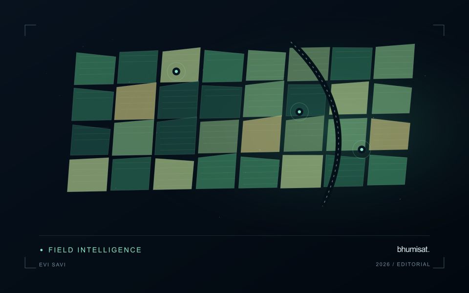
This working guide considers choosing evi, savi and related indices in potato growing fields. The immediate decision is to focus scouting within potato fields. Useful reference evidence includes emergence records, canopy stage and representative plot observations. The case is an illustrative planning context, with assumptions to check against the actual sensor, landscape and project requirements.
The setting: Potato growing fields
Potato monitoring begins with the distinction between the canopy visible from above and the crop component ultimately harvested below ground. Establishment timing, variety, row structure and management can create different canopy patterns across fields. An image service should specify whether it is supporting crop-stage assessment, identifying areas for inspection or estimating a defined production variable. These objectives require different reference measurements and should not be combined into one unqualified vegetation score.
Maintain a field timeline that includes planting, emergence and the operations that can affect canopy appearance. Early observations may contain a large soil contribution, while later observations may show a more continuous canopy. Cloud and shadow contamination, field edges and neighbouring land cover can alter summaries at either stage. Compare observations using suitable quality rules and retain the acquisition dates so that a recent-looking map does not conceal an old measurement.
A field team should collect consistent crop-stage and canopy observations across both flagged and typical areas. Record management context and sampling support rather than relying on an isolated photograph. A vegetation change cannot establish the presence of a specific disease, and a canopy index is not a direct measurement of tuber yield. Evaluate any production model with appropriate harvest data and independent assessment, while keeping the simpler inspection-priority product transparent about what it actually observes.
Choose the index around the landscape
Vegetation indices emphasise selected relationships between spectral measurements. They are alternative views of the same observed surface, not independent diagnoses of a crop. EVI and SAVI were developed to address particular limitations encountered when interpreting vegetation signals, including background and canopy effects. Their usefulness depends on the data and landscape. A workflow should identify which limitation matters in its application before adding another index. Computing many indices without a clear comparison plan can increase complexity while leaving the original question unresolved.
SAVI introduces an adjustment intended to reduce sensitivity to soil brightness when vegetation cover is limited. The adjustment parameter should be chosen deliberately and retained in the processing record. EVI includes additional terms and commonly uses a blue band, making the quality of that measurement relevant to the result. Implementations must use the appropriate reflectance scaling and coefficient conventions. Applying a formula directly to stored integer values without considering offsets and scale factors can produce values that are mathematically calculable yet physically inconsistent.
Test whether the choice improves the decision
Compare candidate indices using the same quality-screened observations, field boundaries and independent evaluation sample. Otherwise a difference in performance might reflect a different set of pixels or dates rather than the index itself. Inspect sparse, intermediate and dense canopy conditions separately. Include soil exposure and recent management operations in the interpretation. A result that appears clearer on a colour map still needs to be tested against the variable of interest or the operational decision the service is expected to support.
The final choice should also account for maintenance and communication. An index that gives a modest improvement but depends on a less reliable band may require additional quality controls. Users should be told which observations were excluded and why a value is missing. Keep the selected method stable during an evaluation period, and version later changes so that historical comparisons remain interpretable. A concise set of well-understood indicators usually supports a stronger service than a long list of unexplained metrics that imply more certainty than the measurements justify.
Budget the complete processing workflow
A processing budget should cover the complete path from source observations to a maintained product. Data access and computing are only part of that path. Include preparation, geographic updates, reference collection, expert review, delivery, and support where those activities belong to the service. A calculation that runs cheaply on a small demonstration can still require substantial effort when the surrounding work is repeated across many locations.
Measure representative tasks rather than assuming that every observation costs the same amount to process. Record data volume, processing time, retry frequency, manual interventions, and the conditions that create unusually demanding cases. Separate fixed setup work from work that grows with the number of observations or users. These records support decisions about batching, caching, storage policy, and the point at which a different processing design becomes worthwhile.
Connect the budget to a defined level of service. Faster delivery, more frequent observation, broader coverage, or more detailed review can each change the resources required. Describe these trade-offs before promising a delivery pattern that the workflow has not demonstrated. Review the budget using operational evidence and preserve enough detail to understand changes between processing versions. The aim is a sustainable service whose resource choices remain aligned with the information that users value.
Match the timing of reference observations
The value of a reference measurement depends partly on how well its timing matches the observation being evaluated. A surface, crop, water body, or instrument state may change between the two measurements. Start by documenting the acquisition time of every source and the period over which the reference observation applies. Avoid treating a date entered during data upload as though it were necessarily the time when the measurement was collected.
Define an acceptable timing relationship for the application. A slowly changing structural feature may tolerate a broader comparison window than a rapidly changing surface condition. The window should be justified by the process being studied and by any available contextual records. If conditions change within that period, consider separating the observations into suitable groups rather than combining them under a single assumption of comparability.
Preserve information about interventions and events between observations. A management operation, rainfall episode, disturbance, or change in sensor configuration can alter the interpretation of a comparison. Record the event and decide whether the pair remains suitable for evaluation. Where the timing mismatch cannot be resolved, describe the comparison as qualified evidence. This is more informative than allowing an uncertain match to influence a performance statistic without explanation.
Bring the evidence back to the decision
A strong interpretation states what was observed, which explanations remain plausible, and what additional evidence would help distinguish them. Avoid presenting a convenient label as a confirmed cause when the measurements support only a broader pattern. Connect the proposed next step to the significance of the decision and the confidence available. This creates an interpretation that a field team, analyst, or project partner can examine, challenge, and improve as further observations become available.
Sources & further reading
Explore the bhumisat spacecraft concept and our vision towards 2030, or return to the journal.