Comparisons through time are valuable only when the observations are sufficiently comparable for the question being asked. A difference between dates can reflect real change, a normal stage in a seasonal cycle, or a difference in how the surface was observed. This perspective examines the reference period, the timing of acquisitions, and the contextual records needed to interpret a sequence. It encourages the use of appropriate baselines rather than treating every previous observation as an equivalent benchmark. The objective is to identify changes that remain meaningful after normal variation and measurement conditions are considered.
This working guide considers turning collected imagery into delivered data in maize production fields. The immediate decision is to prioritise uneven-development scouting. Useful reference evidence includes emergence dates, plant stand notes and field stage. The case is an illustrative planning context, with assumptions to check against the actual sensor, landscape and project requirements.
The setting: Maize production fields
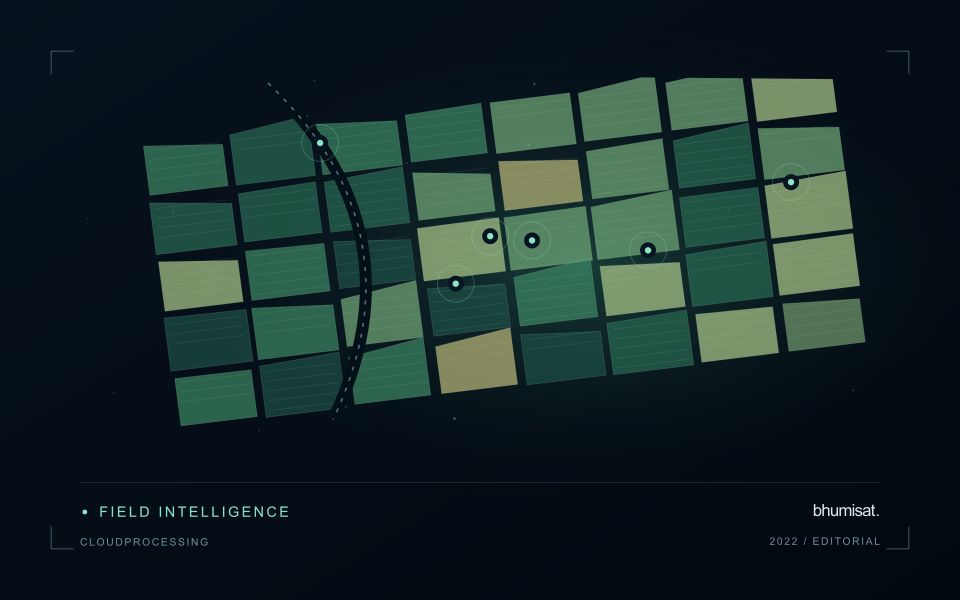
Maize fields can differ in emergence date, variety, plant density and management even within the same growing region. An image comparison is more meaningful when those differences are recorded. Early in the cycle, visible soil and row arrangement can influence a field summary substantially. Later, the canopy may become dense enough that some vegetation measures respond less clearly to additional growth. Interpret the observations in relation to the crop stage and the variable of interest.
Construct a field timeline that marks establishment, important field operations and the dates of usable observations. A decline or delayed increase in a signal can suggest a place to investigate, but several explanations may be possible. Soil conditions, weeds, storm effects and crop timing can produce patterns that require field context. Avoid turning a general anomaly map into a specific diagnosis without measurements that distinguish between these alternatives.
A scouting plan should include representative normal areas as well as the locations ranked most unusual. Record crop stage, stand continuity, visible damage and management information consistently. Production models require their own training and evaluation data, ideally covering different fields and seasons. For operational use, assess whether a satellite-derived priority list helps the field team find relevant conditions efficiently, and report the observation age whenever weather leaves a gap in the current image sequence.
Start with the data that must reach users
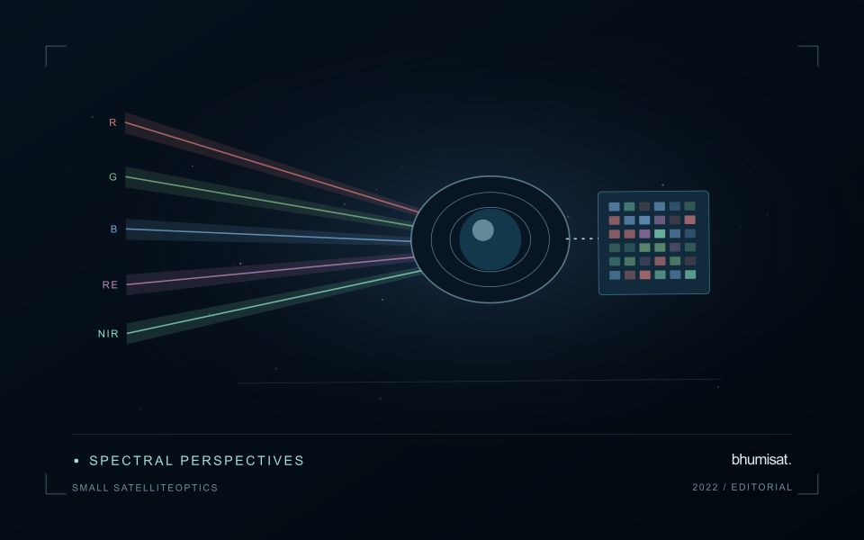
A satellite camera's collection rate and a radio's advertised bit rate do not determine how much useful imagery reaches the ground. The complete data path includes detector output, onboard processing, storage, contact scheduling, transmission and ground processing. Each stage can constrain delivery. Begin with an observation plan and estimate the data it generates, including spectral bands, sampling, encoding, metadata and housekeeping information.
Distinguish raw payload rate from the net rate available for science files. Framing, error control, protocol overhead and operational interruptions reduce effective throughput. Compression can lower volume, but its value depends on scene content and acceptable information loss. Test a representative range of imagery and assess whether any lossy approach alters the measurements needed by the application. A visually pleasing result is not sufficient evidence for quantitative analysis.
Model contacts, storage and recovery together
Ground contacts depend on orbit geometry, station location, visibility constraints and access to the station schedule. The highest rate may be available only during part of a pass. A link budget combines transmitter power, antenna gains, propagation loss, receiver performance and other losses to assess whether the required performance is feasible. Antenna orientation and spacecraft pointing must be consistent with imaging, power generation and other operating demands.
Use a time ordered simulation to track the stored data backlog. Add each planned acquisition and subtract the amount that can actually be delivered during usable contacts. Include missed passes, reduced rates and retransmission policy where relevant. Storage must accommodate plausible disruptions as well as nominal operation. Define priorities and deletion rules before the buffer fills, preserving the metadata needed to identify what was collected and what was lost.
The ground segment needs more than an antenna. It must authenticate commands where applicable, receive and verify files, detect gaps, maintain acquisition records and feed the processing pipeline. Measure latency from observation to the user's usable product, since a successfully received file may still wait for calibration or quality checks. End to end tests should exercise realistic file sizes and interrupted transfers. A sound delivery plan balances collection ambition with energy, contact time and processing capacity, so that an observation schedule produces a dependable flow of usable information.
Maintain the geographic units of analysis
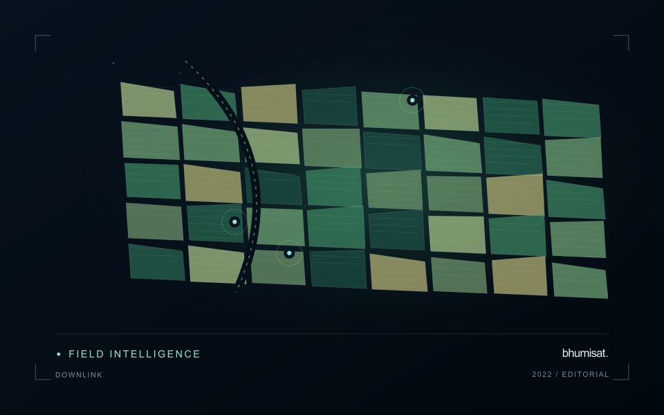
Many observation services summarise measurements within a field, management block, catchment, forest unit, or other mapped boundary. The meaning of that summary depends on whether the boundary accurately represents the unit being discussed. Start with a clear source for the geometry and record its date, coordinate reference, and intended use. A boundary drawn for visual orientation may require additional checking before it becomes a measurement unit.
Inspect overlaps, gaps, narrow fragments, and features that may have changed since mapping. A geometrically valid polygon can still describe an outdated operational unit. Ask the responsible team how divisions, mergers, new infrastructure, and management changes are recorded. Where pixels or reference measurements cross a boundary, define how they are assigned or excluded so that results remain comparable between analysts and processing runs.
Version the boundaries alongside the observations. If a unit changes, preserve a relationship between the previous and revised geometry rather than replacing the history without explanation. Comparisons through time should identify whether they use a constant spatial unit or the operational units valid at each date. This makes it easier to distinguish a change in the measured surface from a change introduced by the geography used to summarise it.
Design an evaluation that reflects deployment
A model evaluation should resemble the conditions in which the model will be used. Start by identifying which relationships the development data share: nearby locations, repeated observations of the same unit, common collection teams, or measurements from a single period. These relationships can make records less independent than they appear. An evaluation that ignores them may test the ability to recognise familiar conditions rather than the ability to operate in a new setting.
Choose a split strategy that matches the intended transfer. Holding out locations, seasons, operational units, or acquisition conditions can answer different questions. Document which question each split is designed to address, and keep the held-out evidence separate while selecting features and tuning the method. Repeatedly inspecting the same evaluation set to improve a model gradually makes that set part of development, even if it retains its original label.
Report results at a scale that is meaningful to the user. A strong average can hide poor performance for important subgroups or unusual conditions. Examine error patterns and retain examples of both successful and unsuccessful predictions. Where the evidence covers only a limited range of conditions, describe that range explicitly. The evaluation then becomes a practical guide to suitable use, further testing, and the collection of additional reference observations.
Bring the evidence back to the decision
A useful comparison preserves the dates, quality conditions, and contextual assumptions behind its baseline. Review unusual results against the actual observation sequence rather than relying entirely on a summary statistic. Where seasonal timing is important, describe how comparable stages were identified. The resulting analysis should help users distinguish an informative change from an expected cycle or an observation artefact, while making gaps and remaining uncertainty visible enough to guide further investigation.
Sources & further reading
Explore the bhumisat spacecraft concept and our vision towards 2030, or return to the journal.