Remote observations show patterns, while practical decisions depend on explaining what those patterns could mean. Interpretation therefore requires more than locating a high or low value on a map. A useful analysis considers the timing of the observation, the physical processes that influence the measurement, and the information available from complementary sources. This perspective separates an observed signal from a proposed explanation and from an action recommended to a user. Keeping those stages distinct makes it easier to investigate alternative causes, communicate ambiguity, and choose a proportionate next step.
This working guide considers turning collected imagery into delivered data across estuarine mixing zones. The immediate decision is to plan sampling across estuarine gradients. Useful reference evidence includes tidal stage, sample timing and water-variable measurements. The case is an illustrative planning context, with assumptions to check against the actual sensor, landscape and project requirements.
Start with the data that must reach users
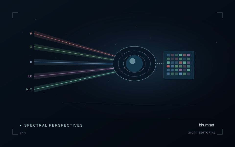
A satellite camera's collection rate and a radio's advertised bit rate do not determine how much useful imagery reaches the ground. The complete data path includes detector output, onboard processing, storage, contact scheduling, transmission and ground processing. Each stage can constrain delivery. Begin with an observation plan and estimate the data it generates, including spectral bands, sampling, encoding, metadata and housekeeping information.
Distinguish raw payload rate from the net rate available for science files. Framing, error control, protocol overhead and operational interruptions reduce effective throughput. Compression can lower volume, but its value depends on scene content and acceptable information loss. Test a representative range of imagery and assess whether any lossy approach alters the measurements needed by the application. A visually pleasing result is not sufficient evidence for quantitative analysis.
Model contacts, storage and recovery together
Ground contacts depend on orbit geometry, station location, visibility constraints and access to the station schedule. The highest rate may be available only during part of a pass. A link budget combines transmitter power, antenna gains, propagation loss, receiver performance and other losses to assess whether the required performance is feasible. Antenna orientation and spacecraft pointing must be consistent with imaging, power generation and other operating demands.
Use a time ordered simulation to track the stored data backlog. Add each planned acquisition and subtract the amount that can actually be delivered during usable contacts. Include missed passes, reduced rates and retransmission policy where relevant. Storage must accommodate plausible disruptions as well as nominal operation. Define priorities and deletion rules before the buffer fills, preserving the metadata needed to identify what was collected and what was lost.
The ground segment needs more than an antenna. It must authenticate commands where applicable, receive and verify files, detect gaps, maintain acquisition records and feed the processing pipeline. Measure latency from observation to the user's usable product, since a successfully received file may still wait for calibration or quality checks. End to end tests should exercise realistic file sizes and interrupted transfers. A sound delivery plan balances collection ambition with energy, contact time and processing capacity, so that an observation schedule produces a dependable flow of usable information.
The setting: Estuarine mixing zones
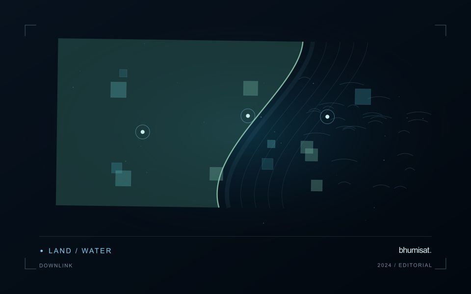
An estuary connects river inflow, coastal water, tidal conditions and complex shorelines. The resulting image pattern may change even when a monitoring team has not altered its methods. A useful design begins with a specific question, such as mapping visible water or investigating a persistent spectral gradient. It should not assume that one relationship describes every part of the estuary or that a single acquisition represents conditions throughout a tidal cycle.
Comparison units should account for channels, shallow margins and locations where land and water are mixed within an observation. Review cloud and atmospheric quality, surface reflection and geometric alignment before interpreting a difference between dates. Tidal and inflow context can help explain the setting but does not replace measurements of the target variable. Preserve the acquisition times and valid areas so that a mapped feature can be evaluated against the conditions under which it was observed.
A validation plan should represent different water types and spatial positions across the mixing zone. Collect the timing and location of samples consistently, and consider whether conditions changed between sampling and acquisition. A spectral boundary may help organise an investigation without proving a particular source or ecological consequence. More specific interpretations require evidence designed for those claims, while an auditable record of observed patterns and sampling priorities can already improve the structure of a monitoring programme.
Check spatial alignment before comparison
A comparison between images, channels, maps, or field measurements assumes that the observations refer to the same locations at a suitable level of precision. Small alignment errors can become especially important near boundaries or narrow features. Before interpreting differences, inspect whether identifiable, stable features agree between the sources. A common coordinate reference is necessary for many workflows, but it does not by itself demonstrate accurate alignment.
Use control features that are appropriate for the observation scale and remain stable across the comparison period. Evaluate alignment in more than one part of the area, because a single location cannot reveal spatially varying distortion. Record the method used to estimate any correction and retain independent features for checking the corrected result. Where surfaces have genuinely changed, avoid using those changes as evidence of an alignment error.
Propagate the implications of remaining misalignment into the analysis. A workflow may exclude boundary pixels, summarise at a broader scale, or qualify interpretations for small features. The choice should follow the application rather than a preference for visually smooth output. Preserve both the original and corrected geographic references, and document resampling decisions so that future users can understand how measurements were moved onto a common spatial framework.
Maintain the geographic units of analysis
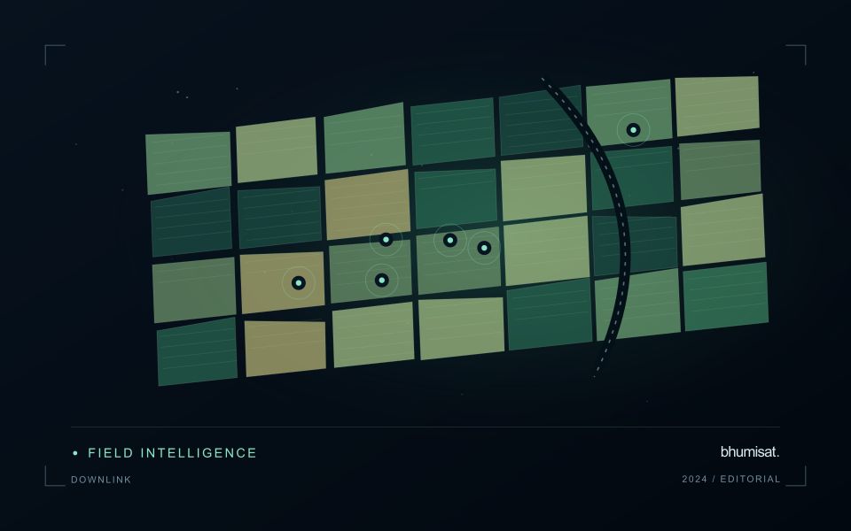
Many observation services summarise measurements within a field, management block, catchment, forest unit, or other mapped boundary. The meaning of that summary depends on whether the boundary accurately represents the unit being discussed. Start with a clear source for the geometry and record its date, coordinate reference, and intended use. A boundary drawn for visual orientation may require additional checking before it becomes a measurement unit.
Inspect overlaps, gaps, narrow fragments, and features that may have changed since mapping. A geometrically valid polygon can still describe an outdated operational unit. Ask the responsible team how divisions, mergers, new infrastructure, and management changes are recorded. Where pixels or reference measurements cross a boundary, define how they are assigned or excluded so that results remain comparable between analysts and processing runs.
Version the boundaries alongside the observations. If a unit changes, preserve a relationship between the previous and revised geometry rather than replacing the history without explanation. Comparisons through time should identify whether they use a constant spatial unit or the operational units valid at each date. This makes it easier to distinguish a change in the measured surface from a change introduced by the geography used to summarise it.
Bring the evidence back to the decision
A strong interpretation states what was observed, which explanations remain plausible, and what additional evidence would help distinguish them. Avoid presenting a convenient label as a confirmed cause when the measurements support only a broader pattern. Connect the proposed next step to the significance of the decision and the confidence available. This creates an interpretation that a field team, analyst, or project partner can examine, challenge, and improve as further observations become available.
Sources & further reading
Explore the bhumisat spacecraft concept and our vision towards 2030, or return to the journal.