A useful observation programme begins with a decision that somebody can act on. Before selecting imagery or instruments, define the area of interest, the people responsible for inspecting it, and the time available for a response. This planning perspective connects remote measurements with the practical questions that shape a survey or monitoring service. The aim is to identify which observations would change a decision, how supporting evidence would be collected, and what should happen when information is incomplete. A clear plan makes later technical choices easier to assess against an operational purpose.
This working guide considers estimating coastal water quality from ocean colour within seasonal wetland areas. The immediate decision is to review changes in inundation and cover. Useful reference evidence includes water presence, vegetation structure and dated site observations. The case is an illustrative planning context, with assumptions to check against the actual sensor, landscape and project requirements.
Identify the quantity behind the colour
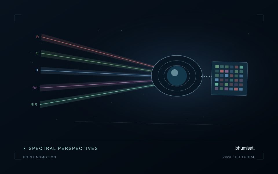
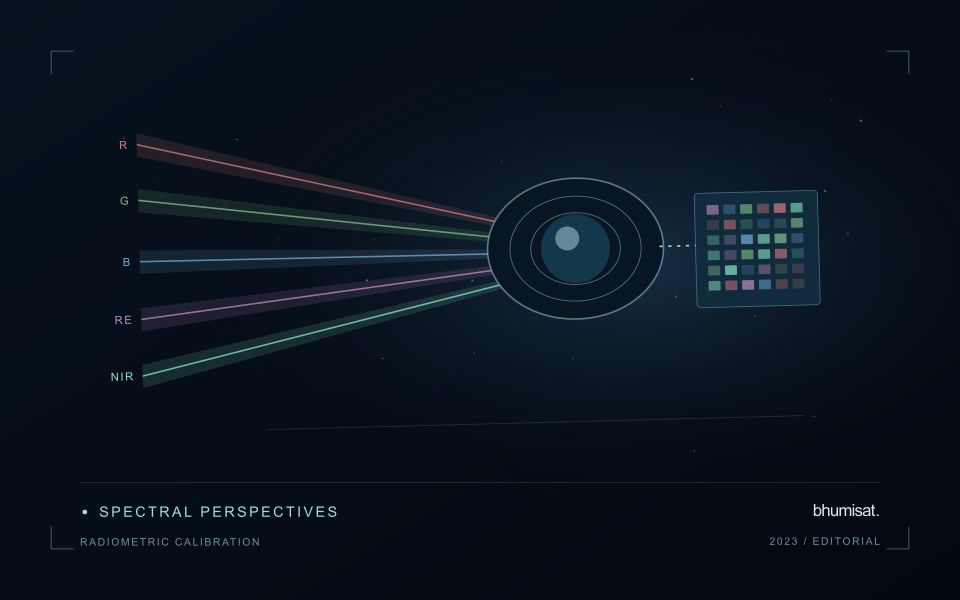
Coastal water colour carries information about materials that absorb and scatter light, including phytoplankton pigments, suspended particles, and dissolved organic matter. A satellite measures radiation reaching the sensor; estimating water quality requires separating the atmospheric contribution and then interpreting the remaining water signal. Specify the target variable and units before choosing an algorithm. Chlorophyll concentration, turbidity, suspended sediment concentration, and water clarity are related in some settings, but they are not interchangeable measurements.
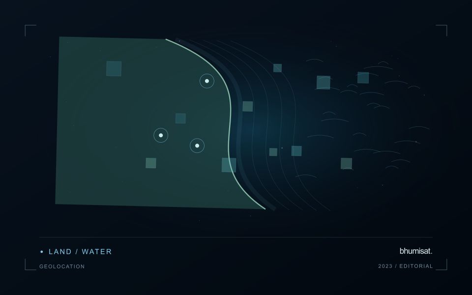
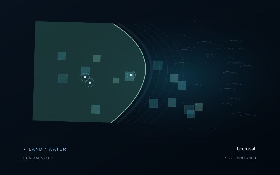
Coasts are especially difficult because several optically active constituents can vary independently. A band ratio calibrated for clear offshore water may fail in a sediment rich estuary. Reflected light from nearby land can contaminate coastal pixels, sun glint can dominate the surface signal, and shallow bottoms can influence apparent colour. Cloud, haze, whitecaps, and mixed land water pixels further reduce usable coverage. Selecting an atmospheric correction method and applying its quality flags are scientific choices, not merely file preparation. Examine spectra and spatial patterns before accepting a plausible looking concentration map.
Match observations to a changing coast
Design validation around the speed of coastal change. Field measurements taken several hours away from the satellite overpass may describe another water mass after tides, currents, or river discharge have shifted conditions. Record sampling time, position, depth, instrument calibration, laboratory methods, and the spatial variability around each station. Satellite pixels integrate an area, while a bottle sample represents a much smaller volume. Use suitable matchups and inspect surrounding pixels rather than pairing every station with the nearest value automatically.
Develop or select retrieval relationships using samples that span the expected range of conditions. Reserve independent data for evaluation and report bias, error, valid sample count, and cases rejected by quality screening. Compare algorithms on the same matchups to avoid misleading differences caused by sampling. Provide acquisition dates, water masks, uncertainty information, and clearly labeled units with every map. A surface optical product does not establish conditions throughout the water column, and a pigment estimate does not by itself identify a harmful species or toxin. Used with field observations and local hydrology, the imagery can reveal spatial gradients and help prioritize where additional sampling is needed.
The setting: Seasonal wetland areas
A seasonal wetland is a changing combination of open water, wet soil, emergent vegetation and drier surfaces. An image feature that separates water from land during one period may behave differently when vegetation becomes denser or the surface changes. Define the mapping objective and its seasonal context carefully. Monitoring visible inundation, describing vegetation change and assessing an ecological outcome require different reference information and should not be merged into one unqualified indicator.
The observation footprint may mix several wetland components, particularly along narrow channels and patchy margins. Optical data can be limited by clouds and by vegetation that obscures water below. Complementary observations can add useful information, but they describe different physical properties and need their own interpretation. Retain dates, quality information and the spatial support used in each result so that a user can judge what the observations actually establish.
Field validation should record water presence and vegetation conditions separately at known locations. Sampling only easily reached dry margins may misrepresent the interior or the range of seasonal states. A change in mapped extent can help select sites for review without explaining its cause. More specific conclusions about habitat condition or management success need measurements aligned with those outcomes. A transparent monitoring record should distinguish observed surface changes from interpretations supported by additional field evidence.
Represent gaps without inventing observations
A monitoring sequence often contains periods without a usable observation. The reason may be cloud, shadow, missing coverage, a failed transfer, or a quality condition that excludes the data. Begin by representing these states explicitly. A missing observation is different from a low measurement, an unchanged surface, or a confirmed absence of the feature being studied. The distinction should survive both the analysis and the presentation of the result.
Define when a temporal gap is acceptable for the intended decision. A workflow may continue using the latest qualified observation, request another source, or suspend an alert until sufficient evidence is available. Whichever response is selected, show the age of the supporting observation. If interpolation is used for a suitable analytical purpose, preserve the distinction between an estimated value and a directly observed measurement, together with the assumptions needed to interpret it.
Review how gaps affect the coverage of the final evaluation. Locations with frequent missing data may differ systematically from those with regular observations. A performance estimate based only on clear, complete records can therefore describe a narrower population than the service is expected to support. Report usable coverage alongside analytical results and use recurring gaps to guide acquisition planning, reference collection, and the selection of complementary observation methods.
Budget the complete processing workflow
A processing budget should cover the complete path from source observations to a maintained product. Data access and computing are only part of that path. Include preparation, geographic updates, reference collection, expert review, delivery, and support where those activities belong to the service. A calculation that runs cheaply on a small demonstration can still require substantial effort when the surrounding work is repeated across many locations.
Measure representative tasks rather than assuming that every observation costs the same amount to process. Record data volume, processing time, retry frequency, manual interventions, and the conditions that create unusually demanding cases. Separate fixed setup work from work that grows with the number of observations or users. These records support decisions about batching, caching, storage policy, and the point at which a different processing design becomes worthwhile.
Connect the budget to a defined level of service. Faster delivery, more frequent observation, broader coverage, or more detailed review can each change the resources required. Describe these trade-offs before promising a delivery pattern that the workflow has not demonstrated. Review the budget using operational evidence and preserve enough detail to understand changes between processing versions. The aim is a sustainable service whose resource choices remain aligned with the information that users value.
Bring the evidence back to the decision
The practical outcome should be a short observation plan that another team can follow. It should name the decision, the required evidence, the responsible roles, and the conditions that trigger a field visit or further analysis. Keep the plan small enough to test, then revise it using the results of real inspections. A useful monitoring workflow improves because its assumptions are examined systematically, and its observations remain connected to decisions throughout the process.
Sources & further reading
Explore the bhumisat spacecraft concept and our vision towards 2030, or return to the journal.