Every observation and interpretation contains uncertainty, but the sources and consequences of that uncertainty differ between applications. Some arise from acquisition conditions, others from reference measurements, processing choices, or the transfer of a model to a new setting. This perspective examines how those sources affect the decision a user is considering. It encourages teams to describe uncertainty in a form that can influence action, rather than adding a generic qualification at the end of a report. The objective is to support proportionate decisions while keeping the limits of the available evidence understandable.
This working guide considers estimating coastal water quality from ocean colour across river floodplain areas. The immediate decision is to locate areas needing flood-impact review. Useful reference evidence includes dated water observations and representative field impact records. The case is an illustrative planning context, with assumptions to check against the actual sensor, landscape and project requirements.
The setting: River floodplain areas
A floodplain contains channels, low-lying fields, settlements, wetlands and surfaces that may be wet or dry under ordinary conditions. A flood-monitoring workflow should distinguish a new observation of water from the baseline distribution expected in that setting. Define the event period and the intended output, such as visible inundation extent or locations for field impact assessment. These products do not automatically establish water depth, damage or the cause of a particular local condition.
Cloud cover can limit optical observations during an event, while vegetation and structures may obscure water at the surface. Other observation types can contribute complementary evidence but require interpretation appropriate to their measurement physics. Compare suitable baseline and event acquisitions, check alignment and preserve the actual observation times. A map assembled from different dates should make those differences clear rather than implying that the whole floodplain was observed simultaneously.
Field validation should record when water or impacts were observed, the location and the area represented by each report. Conditions can change between an image acquisition and a visit, so apparent disagreement may reflect timing rather than a simple mapping error. Sample different land-cover settings and include places outside the mapped extent. A useful product communicates the evidence for observed inundation separately from estimates of damage or operational consequences that require further measurements.
Identify the quantity behind the colour
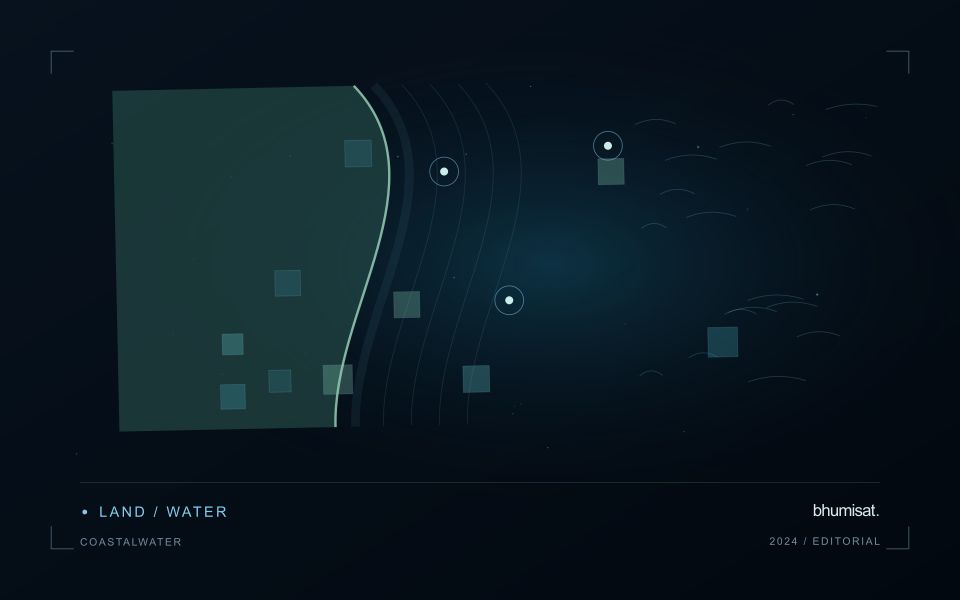
Coastal water colour carries information about materials that absorb and scatter light, including phytoplankton pigments, suspended particles, and dissolved organic matter. A satellite measures radiation reaching the sensor; estimating water quality requires separating the atmospheric contribution and then interpreting the remaining water signal. Specify the target variable and units before choosing an algorithm. Chlorophyll concentration, turbidity, suspended sediment concentration, and water clarity are related in some settings, but they are not interchangeable measurements.
Coasts are especially difficult because several optically active constituents can vary independently. A band ratio calibrated for clear offshore water may fail in a sediment rich estuary. Reflected light from nearby land can contaminate coastal pixels, sun glint can dominate the surface signal, and shallow bottoms can influence apparent colour. Cloud, haze, whitecaps, and mixed land water pixels further reduce usable coverage. Selecting an atmospheric correction method and applying its quality flags are scientific choices, not merely file preparation. Examine spectra and spatial patterns before accepting a plausible looking concentration map.
Match observations to a changing coast
Design validation around the speed of coastal change. Field measurements taken several hours away from the satellite overpass may describe another water mass after tides, currents, or river discharge have shifted conditions. Record sampling time, position, depth, instrument calibration, laboratory methods, and the spatial variability around each station. Satellite pixels integrate an area, while a bottle sample represents a much smaller volume. Use suitable matchups and inspect surrounding pixels rather than pairing every station with the nearest value automatically.
Develop or select retrieval relationships using samples that span the expected range of conditions. Reserve independent data for evaluation and report bias, error, valid sample count, and cases rejected by quality screening. Compare algorithms on the same matchups to avoid misleading differences caused by sampling. Provide acquisition dates, water masks, uncertainty information, and clearly labeled units with every map. A surface optical product does not establish conditions throughout the water column, and a pigment estimate does not by itself identify a harmful species or toxin. Used with field observations and local hydrology, the imagery can reveal spatial gradients and help prioritize where additional sampling is needed.
Locate the uncertainty that matters to the decision
An uncertainty budget is a practical description of where a result could become unreliable. Begin with the observation chain: acquisition, calibration, geographic matching, reference measurements, feature calculation, modelling, and delivery. Identify the assumptions at each stage and ask which could materially change the interpretation. The purpose is not to assign a precise number to every limitation. It is to locate the sources that deserve attention for the intended decision.
Separate limitations that can be measured from those that currently require a qualitative description. Repeated measurements may help characterise variability, while comparisons with independent references can reveal systematic differences. Some uncertainties interact, so combining individual error estimates without examining their relationships can produce a misleading impression of precision. Keep the method of assessment visible and avoid treating an unexamined assumption as though it were a negligible contribution.
Use the budget to prioritise further work. The largest visible source of variation is not always the one whose reduction would most improve the decision. Consider which additional observation, test, or contextual record would change confidence in an actionable way. Revisit the budget when the application, observation source, or deployment conditions change. This turns uncertainty analysis into a guide for improving the workflow rather than a qualification added only after the result has been delivered.
Use observation labels with consistent meanings
A reference label should describe an observation that another person could recognise or reproduce. Broad terms such as good, damaged, or unusual can conceal substantial differences between collection teams. Begin by defining the feature or condition being recorded, the observation unit, and the evidence needed to assign a label. Where possible, distinguish a direct measurement from an interpretation made by the observer.
Provide a short collection guide with examples, boundary cases, and a way to record uncertainty. Train observers using shared cases before relying on independently collected labels. If two observers disagree, preserve the disagreement long enough to understand its cause. It may reveal an unclear definition, a genuinely ambiguous condition, a difference in observation scale, or a problem in matching the reference record to the remote measurement.
Retain the context that makes the label interpretable. Location, time, collection method, observer role, and relevant surface conditions can be essential for later review. Changes to the label scheme should be documented and related to earlier versions where a defensible correspondence exists. Consistent labels do not eliminate uncertainty, but they make it possible to investigate disagreement, evaluate analytical methods, and identify where better definitions or additional measurements would improve the evidence.
Bring the evidence back to the decision
Useful uncertainty communication identifies the limitation, explains how it could affect the result, and connects it to a practical response. Some decisions can proceed with a qualified estimate; others require another observation or an independent check. Preserve uncertainty information through processing and delivery so that it is available at the point of use. This makes the analysis more accountable and gives the team a clearer basis for deciding which additional evidence would most improve the outcome.
Sources & further reading
Explore the bhumisat spacecraft concept and our vision towards 2030, or return to the journal.