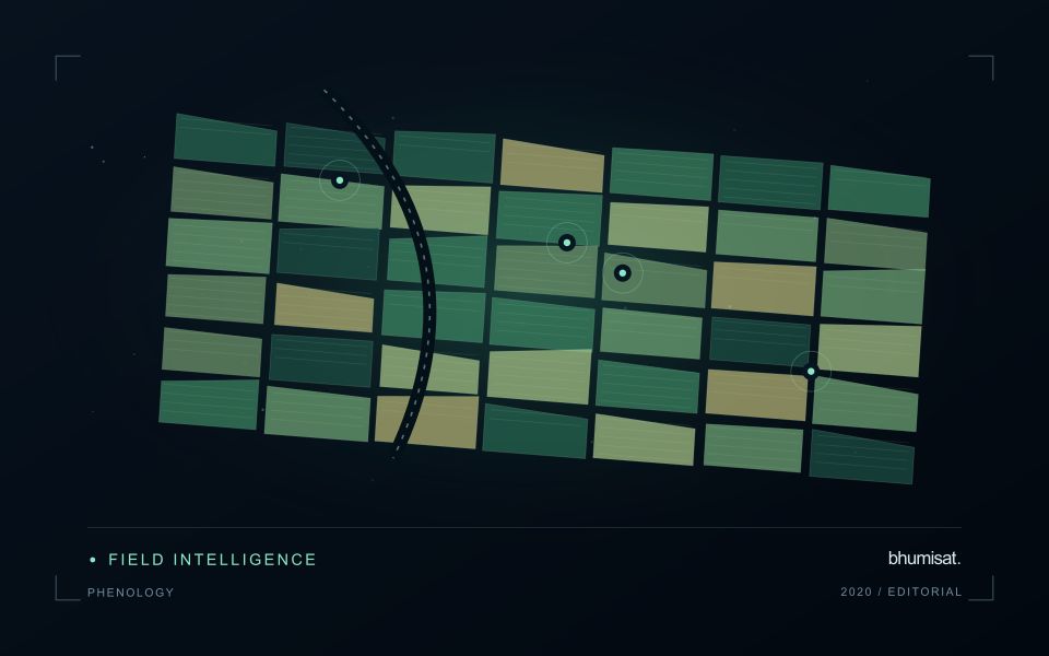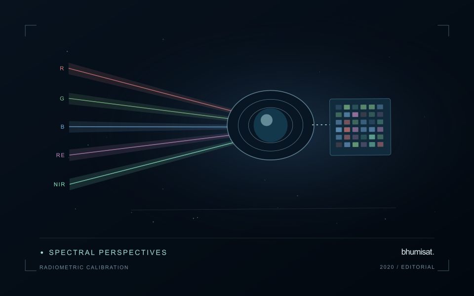
Comparisons through time are valuable only when the observations are sufficiently comparable for the question being asked. A difference between dates can reflect real change, a normal stage in a seasonal cycle, or a difference in how the surface was observed. This perspective examines the reference period, the timing of acquisitions, and the contextual records needed to interpret a sequence. It encourages the use of appropriate baselines rather than treating every previous observation as an equivalent benchmark. The objective is to identify changes that remain meaningful after normal variation and measurement conditions are considered.
This working guide considers cloud and shadow screening for optical imagery in planted timber stands. The immediate decision is to review stand development and harvest boundaries. Useful reference evidence includes planting years, stand management and inventory plot measurements. The case is an illustrative planning context, with assumptions to check against the actual sensor, landscape and project requirements.
A quality mask changes the evidence available
Clouds and their shadows can produce strong changes in optical imagery that have little to do with the condition of the land beneath them. A quality mask identifies observations that should be excluded or treated cautiously for a particular analysis. It is not simply a cosmetic step used to improve an image. The mask determines which measurements contribute to an index, field statistic or time-series model. Its assumptions therefore belong in the analytical record and should remain available when a result is reviewed.
A scene with a low overall cloud percentage can still be unsuitable for a particular farm. Conversely, a partly cloudy scene may contain useful observations over the target fields. Evaluate quality at the area of interest rather than relying only on scene-level metadata. Cloud edges, haze and shadow boundaries can be difficult to classify consistently. Depending on the application, an additional exclusion around a flagged feature may be appropriate. The effect of that choice on usable coverage should be measured instead of hidden.
Check the mask as part of the result
Inspect representative successful and unsuccessful cases before adopting a mask rule across a large archive. Check whether bright soil, roofs, water or dark vegetation are being confused with cloud or shadow. Compare automatic flags with image context and, where available, independent observations. A mask that removes too much valid data can be harmful, while one that retains contamination can create false alerts. The acceptable balance depends on the downstream task and the costs of missed observations and misleading interpretations.
Each delivered field result should state the acquisition date and the fraction of the relevant area supported by valid measurements. If too little remains, a missing result can be more informative than a precise-looking number based on an unrepresentative fragment. Keep observation gaps visible in charts and maps. When the masking method or product version changes, assess how the update affects historical comparability. Treating cloud and shadow screening as part of the evidence chain makes the final agricultural or environmental interpretation easier to audit and more dependable in practice.
The setting: Planted timber stands
A planted timber estate commonly contains stands at different ages and management stages. Newly established areas, closed-canopy stands and recently harvested blocks should not be compared as though their image responses were expected to match. A stand register provides the context for interpreting these differences. Connect boundaries with planting year, species or management group where known, and the operations that could change the canopy during the reporting period.
Remote observations can help organise questions about stand development, harvest extent or unexpected changes within a block. The choice of spatial scale should reflect the stand size and the detail genuinely resolved by the data. Roads, firebreaks, unplanted strips and conservation areas may influence block summaries. When evaluating a trend, inspect image quality and maintain a consistent record of the area contributing valid observations rather than relying on an unqualified average.
Field inventory should record the variables required by the proposed application, such as tree dimensions, stand density or canopy condition, with a clear sampling design. An image-derived cover pattern is not automatically a measurement of timber volume. Relationships used for production or biomass estimation need evaluation across relevant ages and management conditions. A useful initial service may be an auditable stand-development and harvest-monitoring workflow whose mapped observations can be checked against operation records and independent field evidence.
Stratify forest reference observations
Forest landscapes can contain substantial variation in structure, composition, management history, and observation conditions. A reference plan should identify the forms of variation that matter to the intended analysis. Start with a clear target population and use available information to define meaningful strata. The objective is to represent the conditions in which the method will be used, rather than collecting only the most accessible or visually uniform examples.
Match the reference unit to the scale of the remote measurement. A field plot, an individual tree observation, and an image pixel can describe different portions of the canopy and ground. Record plot geometry, position, measurement time, and the procedures used to handle boundaries or incomplete coverage. Where geographic uncertainty is important relative to plot size, evaluate its potential effect before treating a difference between sources as a failure of the analytical method.
Keep the estimation and evaluation questions distinct. Reference measurements used to fit a relationship do not automatically provide an independent test of that relationship. Consider holding out suitable locations or forest conditions when evaluating transfer. Report the range of structure and conditions represented by the evidence, together with important gaps. A stratified reference programme becomes useful when it supports a clear interpretation of where a result is well supported and where further observations are required.
Design an evaluation that reflects deployment
A model evaluation should resemble the conditions in which the model will be used. Start by identifying which relationships the development data share: nearby locations, repeated observations of the same unit, common collection teams, or measurements from a single period. These relationships can make records less independent than they appear. An evaluation that ignores them may test the ability to recognise familiar conditions rather than the ability to operate in a new setting.
Choose a split strategy that matches the intended transfer. Holding out locations, seasons, operational units, or acquisition conditions can answer different questions. Document which question each split is designed to address, and keep the held-out evidence separate while selecting features and tuning the method. Repeatedly inspecting the same evaluation set to improve a model gradually makes that set part of development, even if it retains its original label.
Report results at a scale that is meaningful to the user. A strong average can hide poor performance for important subgroups or unusual conditions. Examine error patterns and retain examples of both successful and unsuccessful predictions. Where the evidence covers only a limited range of conditions, describe that range explicitly. The evaluation then becomes a practical guide to suitable use, further testing, and the collection of additional reference observations.
Bring the evidence back to the decision
A useful comparison preserves the dates, quality conditions, and contextual assumptions behind its baseline. Review unusual results against the actual observation sequence rather than relying entirely on a summary statistic. Where seasonal timing is important, describe how comparable stages were identified. The resulting analysis should help users distinguish an informative change from an expected cycle or an observation artefact, while making gaps and remaining uncertainty visible enough to guide further investigation.
Sources & further reading
Explore the bhumisat spacecraft concept and our vision towards 2030, or return to the journal.