A workflow that succeeds on a small study area may encounter different constraints when the number of observations, locations, or users increases. Scaling requires attention to processing capacity, data organisation, reference coverage, and the effort needed to review results. This perspective looks beyond whether a calculation can run on a larger dataset. It asks whether the complete service can preserve its meaning, quality, and delivery commitments as its scope expands. The objective is a design that identifies bottlenecks early and increases throughput without silently weakening the evidence available to users.
This working guide considers cloud and shadow screening for optical imagery along shallow reef-adjacent coasts. The immediate decision is to select coastal habitat survey areas. Useful reference evidence includes water conditions, survey timing and mapped substrate observations. The case is an illustrative planning context, with assumptions to check against the actual sensor, landscape and project requirements.
A quality mask changes the evidence available
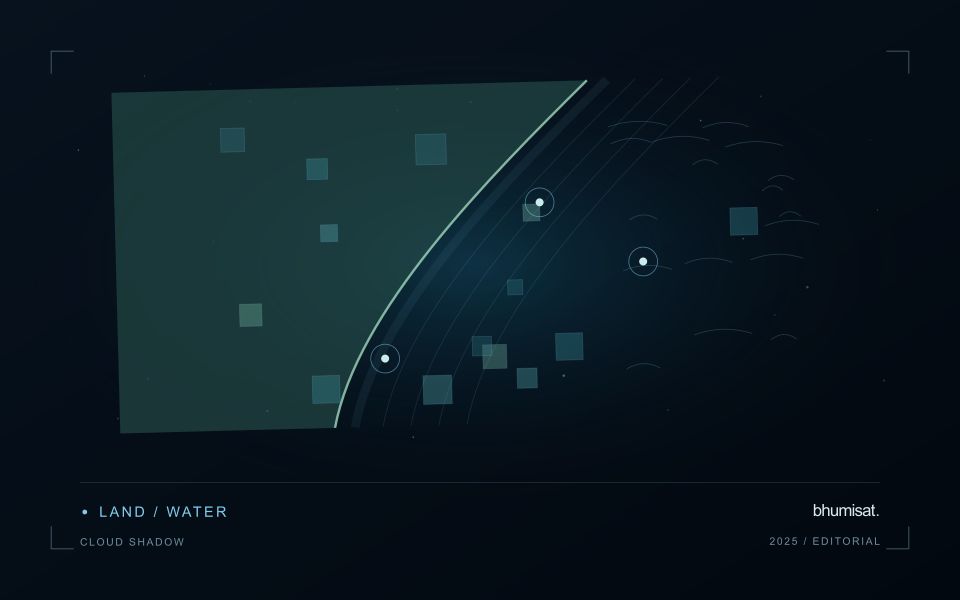
Clouds and their shadows can produce strong changes in optical imagery that have little to do with the condition of the land beneath them. A quality mask identifies observations that should be excluded or treated cautiously for a particular analysis. It is not simply a cosmetic step used to improve an image. The mask determines which measurements contribute to an index, field statistic or time-series model. Its assumptions therefore belong in the analytical record and should remain available when a result is reviewed.
A scene with a low overall cloud percentage can still be unsuitable for a particular farm. Conversely, a partly cloudy scene may contain useful observations over the target fields. Evaluate quality at the area of interest rather than relying only on scene-level metadata. Cloud edges, haze and shadow boundaries can be difficult to classify consistently. Depending on the application, an additional exclusion around a flagged feature may be appropriate. The effect of that choice on usable coverage should be measured instead of hidden.
Check the mask as part of the result
Inspect representative successful and unsuccessful cases before adopting a mask rule across a large archive. Check whether bright soil, roofs, water or dark vegetation are being confused with cloud or shadow. Compare automatic flags with image context and, where available, independent observations. A mask that removes too much valid data can be harmful, while one that retains contamination can create false alerts. The acceptable balance depends on the downstream task and the costs of missed observations and misleading interpretations.
Each delivered field result should state the acquisition date and the fraction of the relevant area supported by valid measurements. If too little remains, a missing result can be more informative than a precise-looking number based on an unrepresentative fragment. Keep observation gaps visible in charts and maps. When the masking method or product version changes, assess how the update affects historical comparability. Treating cloud and shadow screening as part of the evidence chain makes the final agricultural or environmental interpretation easier to audit and more dependable in practice.
The setting: Shallow reef-adjacent coasts
A shallow coastal image can contain a mixture of water-column effects, bottom reflectance, surface reflection and adjacent land. The contribution of the seabed depends on conditions that vary across space and time. A monitoring task should therefore identify what can reasonably be observed at the selected scale. Mapping broad substrate patterns or selecting survey locations is different from diagnosing the condition of individual coral colonies or other small habitat features.
Review water clarity, depth context where available, cloud, atmospheric quality and sun glint before interpreting a spectral difference. Changes in the water above the bottom may alter the image without a corresponding change in the substrate. Shorelines and narrow reef features are also sensitive to mixed pixels and alignment. Comparisons should retain their acquisition dates and processing assumptions so that users can understand what environmental conditions support the proposed interpretation.
Field surveys should document the area represented by each observation and distinguish substrate descriptions from measurements of biological condition. Survey timing and water conditions matter when relating those records to imagery. A broad remotely sensed class cannot validate every feature inside its footprint. Use representative and independent assessment locations where possible, and communicate where the result supports a landscape-scale interpretation or a survey priority rather than a fine-scale ecological conclusion.
Translate the decision into observation requirements
Start with the decision that the information is intended to support. Describe the geographic unit, the time available for acting, and the consequence of an incorrect interpretation. A requirement such as detecting an unusual pattern across management blocks is different from identifying its cause. Keeping that distinction explicit helps a team select measurements that are relevant to the application and prevents later evaluation from drifting towards whatever result happens to be easiest to demonstrate.
Build a compact requirements matrix linking each decision to the evidence needed, the proposed observation source, and an acceptance condition. Include geographic accuracy, temporal relevance, quality screening, and the context required for interpretation. The matrix should also identify the evidence used to justify each requirement. An engineering preference or a convenient data source can inform a study, but neither should silently replace a documented information need.
Review the matrix with the people who will use the result. Ask how their response would change when information is delayed, incomplete, or uncertain. Record unresolved requirements as questions for a pilot rather than converting them into confident specifications. This produces a practical framework for comparing technical options, designing tests, and explaining why an observation is useful to the intended workflow.
Connect observations within a catchment
Water-related observations often depend on processes beyond the immediate pixel or sampling location. Begin by identifying the geographic relationships that are relevant to the question: upstream areas, connected drainage paths, contributing land uses, and the receiving water body. A local pattern may be easier to interpret when placed within that wider setting. The catchment boundary is a useful organising unit, but its suitability should be checked against the process and observation scale.
Combine the remote observation with contextual records that can help explain its timing and spatial pattern. Rainfall, water level, land management, and known interventions can influence what is observed. Preserve the dates and geographic meaning of those records rather than treating them as timeless attributes. Where drainage connections are uncertain or change with conditions, state the limitation and consider whether additional mapping or reference observations would materially improve the interpretation.
Plan reference sampling across locations that distinguish plausible explanations. A set of measurements concentrated at an easily accessible outlet may provide a different view from one that also represents tributaries, source areas, and contrasting conditions. Document how each location contributes to the evaluation. Interpret spatial agreement with care, because connected observations can share influences and may not provide independent evidence. The resulting workflow should connect local measurements with a defensible account of the wider system they help describe.
Bring the evidence back to the decision
Expansion should be guided by measured workload, visible quality conditions, and an understanding of which tasks require expert attention. Test the workflow under representative data volumes before treating a successful demonstration as evidence of operational capacity. Preserve a route for investigating individual observations even when most processing is automated. A scalable service keeps its results traceable and useful as it grows, with clear choices about where to automate, where to review, and where to invest in additional evidence.
Sources & further reading
Explore the bhumisat spacecraft concept and our vision towards 2030, or return to the journal.