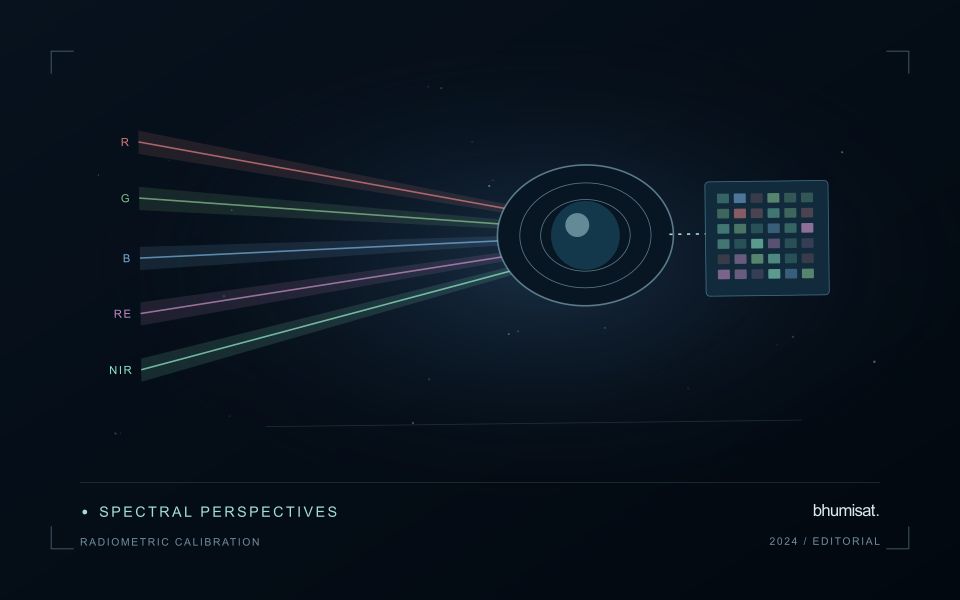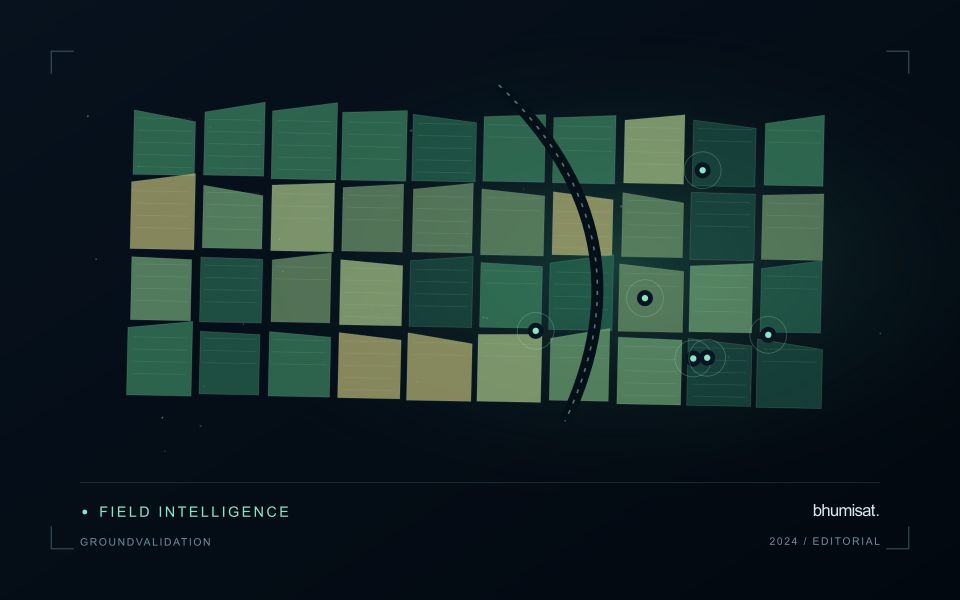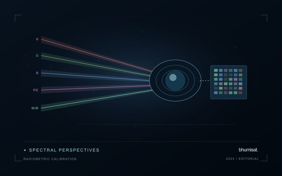
A convincing image can still contain measurements that are unsuitable for a particular task. Quality control asks whether the inputs, transformations, and outputs meet the requirements of the intended application. This perspective follows evidence through the workflow, from acquisition metadata and reference observations to the final interpretation. It encourages teams to define acceptance conditions before seeing the result, rather than adjusting them to favour a preferred conclusion. The purpose is a repeatable way to distinguish usable observations, observations requiring qualification, and observations that should be excluded from a decision.
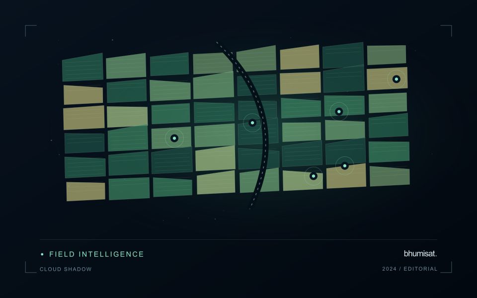
This working guide considers cloud and shadow screening for optical imagery in open-field tomato production. The immediate decision is to select tomato rows for crop review. Useful reference evidence includes transplanting dates, canopy observations and field management notes. The case is an illustrative planning context, with assumptions to check against the actual sensor, landscape and project requirements.
A quality mask changes the evidence available
Clouds and their shadows can produce strong changes in optical imagery that have little to do with the condition of the land beneath them. A quality mask identifies observations that should be excluded or treated cautiously for a particular analysis. It is not simply a cosmetic step used to improve an image. The mask determines which measurements contribute to an index, field statistic or time-series model. Its assumptions therefore belong in the analytical record and should remain available when a result is reviewed.
A scene with a low overall cloud percentage can still be unsuitable for a particular farm. Conversely, a partly cloudy scene may contain useful observations over the target fields. Evaluate quality at the area of interest rather than relying only on scene-level metadata. Cloud edges, haze and shadow boundaries can be difficult to classify consistently. Depending on the application, an additional exclusion around a flagged feature may be appropriate. The effect of that choice on usable coverage should be measured instead of hidden.
Check the mask as part of the result
Inspect representative successful and unsuccessful cases before adopting a mask rule across a large archive. Check whether bright soil, roofs, water or dark vegetation are being confused with cloud or shadow. Compare automatic flags with image context and, where available, independent observations. A mask that removes too much valid data can be harmful, while one that retains contamination can create false alerts. The acceptable balance depends on the downstream task and the costs of missed observations and misleading interpretations.
Each delivered field result should state the acquisition date and the fraction of the relevant area supported by valid measurements. If too little remains, a missing result can be more informative than a precise-looking number based on an unrepresentative fragment. Keep observation gaps visible in charts and maps. When the masking method or product version changes, assess how the update affects historical comparability. Treating cloud and shadow screening as part of the evidence chain makes the final agricultural or environmental interpretation easier to audit and more dependable in practice.
The setting: Open-field tomato production
Open-field tomato production can involve short management cycles, staggered planting and repeated operations within neighbouring parcels. The field calendar is therefore central to interpreting a satellite observation. Newly transplanted plants, established rows and areas nearing the end of production can show different responses for ordinary reasons. Record the planted area and the relevant management unit carefully, particularly where a commercial holding contains several crops or planting stages at the same time.
The image footprint may mix plants with soil, mulch, access routes and irrigation infrastructure. Determine whether the spatial resolution supports the intended row-level interpretation or whether a broader field summary is more appropriate. Examine the quality and age of observations before proposing a management use that depends on rapid response. A monitoring workflow should communicate when cloud gaps or the acquisition schedule leave insufficient current evidence for that decision.
Validation should document crop stage, canopy continuity, recent operations and the area represented by each sample. Field staff may use a mapped anomaly to choose an inspection location, but the subsequent diagnosis requires suitable observations and expertise. If production or quality is the target, collect reference information for those outcomes rather than assuming that greener vegetation implies more marketable fruit. The evaluation should measure whether the product improves a defined scouting or management process.
Maintain the geographic units of analysis
Many observation services summarise measurements within a field, management block, catchment, forest unit, or other mapped boundary. The meaning of that summary depends on whether the boundary accurately represents the unit being discussed. Start with a clear source for the geometry and record its date, coordinate reference, and intended use. A boundary drawn for visual orientation may require additional checking before it becomes a measurement unit.
Inspect overlaps, gaps, narrow fragments, and features that may have changed since mapping. A geometrically valid polygon can still describe an outdated operational unit. Ask the responsible team how divisions, mergers, new infrastructure, and management changes are recorded. Where pixels or reference measurements cross a boundary, define how they are assigned or excluded so that results remain comparable between analysts and processing runs.
Version the boundaries alongside the observations. If a unit changes, preserve a relationship between the previous and revised geometry rather than replacing the history without explanation. Comparisons through time should identify whether they use a constant spatial unit or the operational units valid at each date. This makes it easier to distinguish a change in the measured surface from a change introduced by the geography used to summarise it.
Design an evaluation that reflects deployment
A model evaluation should resemble the conditions in which the model will be used. Start by identifying which relationships the development data share: nearby locations, repeated observations of the same unit, common collection teams, or measurements from a single period. These relationships can make records less independent than they appear. An evaluation that ignores them may test the ability to recognise familiar conditions rather than the ability to operate in a new setting.
Choose a split strategy that matches the intended transfer. Holding out locations, seasons, operational units, or acquisition conditions can answer different questions. Document which question each split is designed to address, and keep the held-out evidence separate while selecting features and tuning the method. Repeatedly inspecting the same evaluation set to improve a model gradually makes that set part of development, even if it retains its original label.
Report results at a scale that is meaningful to the user. A strong average can hide poor performance for important subgroups or unusual conditions. Examine error patterns and retain examples of both successful and unsuccessful predictions. Where the evidence covers only a limited range of conditions, describe that range explicitly. The evaluation then becomes a practical guide to suitable use, further testing, and the collection of additional reference observations.
Bring the evidence back to the decision
Quality control is most useful when its results travel with the information being delivered. Preserve the reasons for accepting or rejecting an observation, and expose limitations that could change the user's interpretation. Review recurring failures as clues about the design of the workflow. A clear quality record supports consistent comparisons between operators and processing versions, while helping the team decide whether a problem originates in acquisition, preparation, interpretation, or the underlying observation requirements.
Sources & further reading
Explore the bhumisat spacecraft concept and our vision towards 2030, or return to the journal.