Remote observations show patterns, while practical decisions depend on explaining what those patterns could mean. Interpretation therefore requires more than locating a high or low value on a map. A useful analysis considers the timing of the observation, the physical processes that influence the measurement, and the information available from complementary sources. This perspective separates an observed signal from a proposed explanation and from an action recommended to a user. Keeping those stages distinct makes it easier to investigate alternative causes, communicate ambiguity, and choose a proportionate next step.
This working guide considers cloud and shadow screening for optical imagery across estuarine mixing zones. The immediate decision is to plan sampling across estuarine gradients. Useful reference evidence includes tidal stage, sample timing and water-variable measurements. The case is an illustrative planning context, with assumptions to check against the actual sensor, landscape and project requirements.
The setting: Estuarine mixing zones
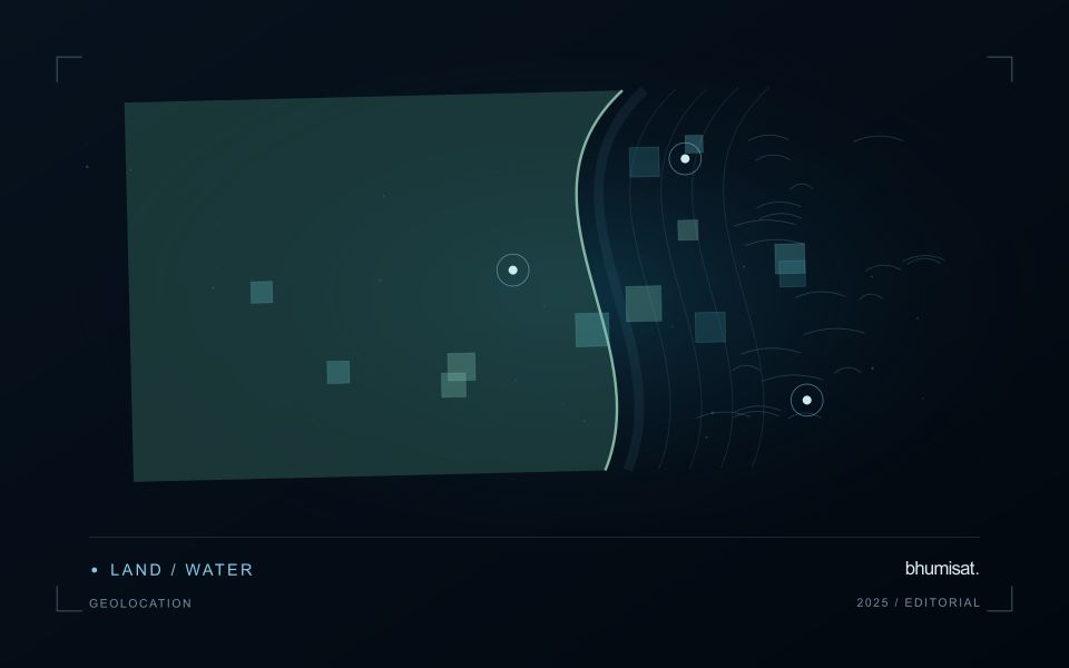
An estuary connects river inflow, coastal water, tidal conditions and complex shorelines. The resulting image pattern may change even when a monitoring team has not altered its methods. A useful design begins with a specific question, such as mapping visible water or investigating a persistent spectral gradient. It should not assume that one relationship describes every part of the estuary or that a single acquisition represents conditions throughout a tidal cycle.
Comparison units should account for channels, shallow margins and locations where land and water are mixed within an observation. Review cloud and atmospheric quality, surface reflection and geometric alignment before interpreting a difference between dates. Tidal and inflow context can help explain the setting but does not replace measurements of the target variable. Preserve the acquisition times and valid areas so that a mapped feature can be evaluated against the conditions under which it was observed.
A validation plan should represent different water types and spatial positions across the mixing zone. Collect the timing and location of samples consistently, and consider whether conditions changed between sampling and acquisition. A spectral boundary may help organise an investigation without proving a particular source or ecological consequence. More specific interpretations require evidence designed for those claims, while an auditable record of observed patterns and sampling priorities can already improve the structure of a monitoring programme.
A quality mask changes the evidence available
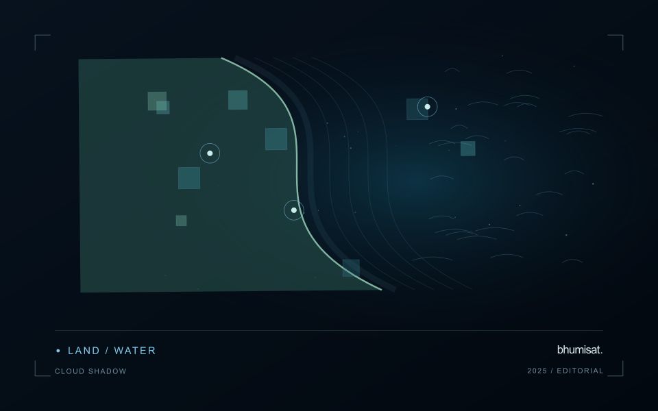
Clouds and their shadows can produce strong changes in optical imagery that have little to do with the condition of the land beneath them. A quality mask identifies observations that should be excluded or treated cautiously for a particular analysis. It is not simply a cosmetic step used to improve an image. The mask determines which measurements contribute to an index, field statistic or time-series model. Its assumptions therefore belong in the analytical record and should remain available when a result is reviewed.
A scene with a low overall cloud percentage can still be unsuitable for a particular farm. Conversely, a partly cloudy scene may contain useful observations over the target fields. Evaluate quality at the area of interest rather than relying only on scene-level metadata. Cloud edges, haze and shadow boundaries can be difficult to classify consistently. Depending on the application, an additional exclusion around a flagged feature may be appropriate. The effect of that choice on usable coverage should be measured instead of hidden.
Check the mask as part of the result
Inspect representative successful and unsuccessful cases before adopting a mask rule across a large archive. Check whether bright soil, roofs, water or dark vegetation are being confused with cloud or shadow. Compare automatic flags with image context and, where available, independent observations. A mask that removes too much valid data can be harmful, while one that retains contamination can create false alerts. The acceptable balance depends on the downstream task and the costs of missed observations and misleading interpretations.
Each delivered field result should state the acquisition date and the fraction of the relevant area supported by valid measurements. If too little remains, a missing result can be more informative than a precise-looking number based on an unrepresentative fragment. Keep observation gaps visible in charts and maps. When the masking method or product version changes, assess how the update affects historical comparability. Treating cloud and shadow screening as part of the evidence chain makes the final agricultural or environmental interpretation easier to audit and more dependable in practice.
Match the timing of reference observations
The value of a reference measurement depends partly on how well its timing matches the observation being evaluated. A surface, crop, water body, or instrument state may change between the two measurements. Start by documenting the acquisition time of every source and the period over which the reference observation applies. Avoid treating a date entered during data upload as though it were necessarily the time when the measurement was collected.
Define an acceptable timing relationship for the application. A slowly changing structural feature may tolerate a broader comparison window than a rapidly changing surface condition. The window should be justified by the process being studied and by any available contextual records. If conditions change within that period, consider separating the observations into suitable groups rather than combining them under a single assumption of comparability.
Preserve information about interventions and events between observations. A management operation, rainfall episode, disturbance, or change in sensor configuration can alter the interpretation of a comparison. Record the event and decide whether the pair remains suitable for evaluation. Where the timing mismatch cannot be resolved, describe the comparison as qualified evidence. This is more informative than allowing an uncertain match to influence a performance statistic without explanation.
Define a representative reference sample
A reference sample should represent the situations in which a method will be used. Begin by defining the target population: locations, time periods, management conditions, surface types, or instrument states that belong within the intended application. A collection of convenient observations may be valuable for exploration, but it does not automatically support conclusions about that wider population. Make the scope of the sample visible before calculating a summary of performance.
Consider a stratified design when important conditions are unevenly represented. Relevant strata might include different landscape types, developmental stages, observation quality levels, or ranges of the variable being estimated. Choose sample locations within those groups using a documented rule, and retain the information needed to understand their selection. Where access restrictions affect the sample, record the excluded conditions so that the limits of the resulting evaluation remain clear.
Keep development and evaluation evidence separate where the purpose of the study requires an independent test. Nearby observations or repeated measurements can share information, so a random split of individual records may overstate independence. A split organised by location, period, or operational unit can provide a more demanding comparison. The appropriate design follows the intended deployment, the structure of the observations, and the errors that matter to the user.
Bring the evidence back to the decision
A strong interpretation states what was observed, which explanations remain plausible, and what additional evidence would help distinguish them. Avoid presenting a convenient label as a confirmed cause when the measurements support only a broader pattern. Connect the proposed next step to the significance of the decision and the confidence available. This creates an interpretation that a field team, analyst, or project partner can examine, challenge, and improve as further observations become available.
Sources & further reading
Explore the bhumisat spacecraft concept and our vision towards 2030, or return to the journal.