Remote observations show patterns, while practical decisions depend on explaining what those patterns could mean. Interpretation therefore requires more than locating a high or low value on a map. A useful analysis considers the timing of the observation, the physical processes that influence the measurement, and the information available from complementary sources. This perspective separates an observed signal from a proposed explanation and from an action recommended to a user. Keeping those stages distinct makes it easier to investigate alternative causes, communicate ambiguity, and choose a proportionate next step.
This working guide considers viewing geometry and brdf effects along river water corridors. The immediate decision is to prioritise river reaches for sampling. Useful reference evidence includes sampling time, river stage and reach-specific water observations. The case is an illustrative planning context, with assumptions to check against the actual sensor, landscape and project requirements.
The observed surface has a direction-dependent response
A surface does not necessarily reflect incoming light equally in every direction. Its measured brightness can change as the positions of the Sun, surface and sensor change, even when the surface itself is similar. The bidirectional reflectance distribution function provides a framework for describing this directional behaviour. In practical image analysis, the relevant lesson is that a difference between observations may contain a geometry effect as well as a real surface change. Canopy structure, shadows and surface roughness can all influence that relationship.
The magnitude and pattern of a geometry effect depend on the landscape and spectral measurement. A row crop, closed forest and exposed soil need not behave in the same way. Terrain introduces another layer because slope and aspect alter local illumination. A simple brightness adjustment is not automatically an adequate solution. A workflow should first identify the type of comparison it needs and whether the available product already includes a relevant normalisation. Applying an additional correction without understanding prior processing can create a new inconsistency.
Normalise geometry with a clear purpose
Geometry normalisation uses a model or adjustment to express observations under a more consistent reference condition. It is an approximation designed for a defined purpose, and its performance should be checked rather than assumed. Keep the input geometry, model assumptions and processing version where they are available. Compare representative surfaces before and after the adjustment. A useful test examines whether the correction reduces systematic variation in stable areas while preserving changes that are supported independently by management records or field observations.
For an agricultural service, the importance of this effect depends on the size of the change being interpreted. A subtle trend can be more sensitive to residual geometry variation than a major harvest event. Evaluate whether an apparent improvement in a time series survives across seasons and fields, including those with different canopy arrangements. Retain a clear explanation of what has been normalised and what remains uncertain. Viewing geometry becomes manageable when it is treated as part of the measurement context instead of being attributed silently to crop condition or land-cover change.
The setting: River water corridors
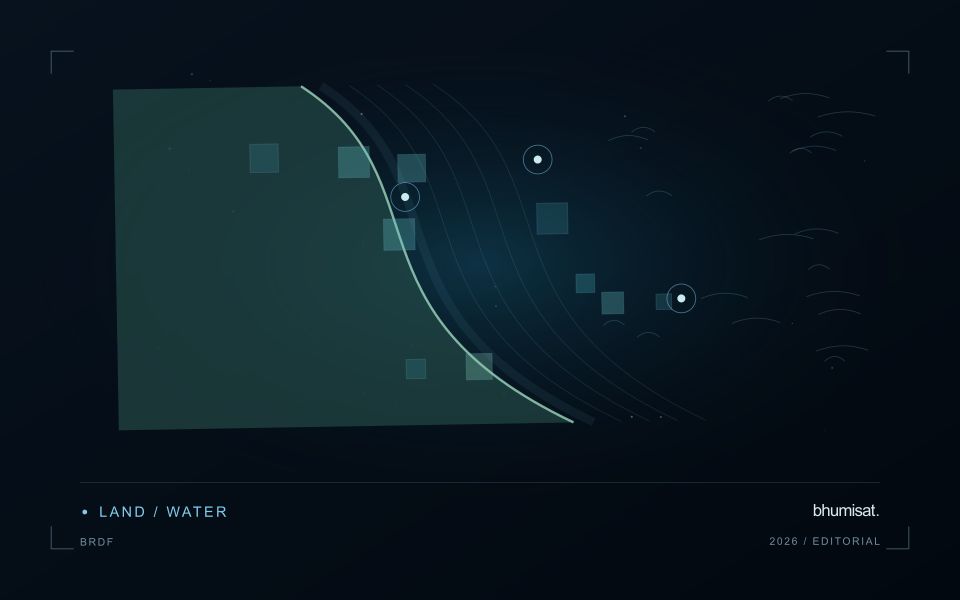
A river corridor can vary quickly in width, bank exposure, flow conditions and the surrounding land cover. A remotely observed reach may include water, sediment, vegetation and structures within the same footprint. Define the monitoring question before choosing an interpretation scale. Mapping the position of visible water, investigating a colour change and estimating a particular water-quality variable are different tasks, even where they draw on the same acquisition.
Spatial resolution and geometric alignment are critical for narrow reaches. A small offset can change how much bank or vegetation contributes to a measurement. Cloud, shadow, surface reflection and adjacency effects can further complicate optical interpretation. Compare suitable acquisitions and retain the exact dates supporting each reach summary. Where river conditions change rapidly, consider whether the available observation frequency is sufficient for the decision the service is intended to support.
Field sampling should identify the sampled reach, location and collection time, together with river conditions that affect comparability. A single bank-side sample may not describe the full width or a downstream reach observed at another time. A spectral anomaly can help select an investigation site without establishing its cause. More specific claims require a validated relationship with representative measurements, while a transparent water and reach inventory can already make a sampling programme more systematic.
Check spatial alignment before comparison
A comparison between images, channels, maps, or field measurements assumes that the observations refer to the same locations at a suitable level of precision. Small alignment errors can become especially important near boundaries or narrow features. Before interpreting differences, inspect whether identifiable, stable features agree between the sources. A common coordinate reference is necessary for many workflows, but it does not by itself demonstrate accurate alignment.
Use control features that are appropriate for the observation scale and remain stable across the comparison period. Evaluate alignment in more than one part of the area, because a single location cannot reveal spatially varying distortion. Record the method used to estimate any correction and retain independent features for checking the corrected result. Where surfaces have genuinely changed, avoid using those changes as evidence of an alignment error.
Propagate the implications of remaining misalignment into the analysis. A workflow may exclude boundary pixels, summarise at a broader scale, or qualify interpretations for small features. The choice should follow the application rather than a preference for visually smooth output. Preserve both the original and corrected geographic references, and document resampling decisions so that future users can understand how measurements were moved onto a common spatial framework.
Locate the uncertainty that matters to the decision
An uncertainty budget is a practical description of where a result could become unreliable. Begin with the observation chain: acquisition, calibration, geographic matching, reference measurements, feature calculation, modelling, and delivery. Identify the assumptions at each stage and ask which could materially change the interpretation. The purpose is not to assign a precise number to every limitation. It is to locate the sources that deserve attention for the intended decision.
Separate limitations that can be measured from those that currently require a qualitative description. Repeated measurements may help characterise variability, while comparisons with independent references can reveal systematic differences. Some uncertainties interact, so combining individual error estimates without examining their relationships can produce a misleading impression of precision. Keep the method of assessment visible and avoid treating an unexamined assumption as though it were a negligible contribution.
Use the budget to prioritise further work. The largest visible source of variation is not always the one whose reduction would most improve the decision. Consider which additional observation, test, or contextual record would change confidence in an actionable way. Revisit the budget when the application, observation source, or deployment conditions change. This turns uncertainty analysis into a guide for improving the workflow rather than a qualification added only after the result has been delivered.
Bring the evidence back to the decision
A strong interpretation states what was observed, which explanations remain plausible, and what additional evidence would help distinguish them. Avoid presenting a convenient label as a confirmed cause when the measurements support only a broader pattern. Connect the proposed next step to the significance of the decision and the confidence available. This creates an interpretation that a field team, analyst, or project partner can examine, challenge, and improve as further observations become available.
Sources & further reading
Explore the bhumisat spacecraft concept and our vision towards 2030, or return to the journal.