An analytical result becomes operational information only when the receiving team can understand it and use it within existing responsibilities. Handoffs often fail because assumptions that were obvious to the analyst are absent from the delivered product. This perspective considers the information needed at that boundary: acquisition time, processing status, geographic scope, quality qualifications, and the action expected from the recipient. It also asks how corrections and feedback should return to the producing team. A dependable handoff creates a shared understanding of the result, rather than merely transferring a file.
This working guide considers viewing geometry and brdf effects in cotton production fields. The immediate decision is to prioritise cotton field scouting. Useful reference evidence includes planting dates, growth stage and canopy observations. The case is an illustrative planning context, with assumptions to check against the actual sensor, landscape and project requirements.
The observed surface has a direction-dependent response
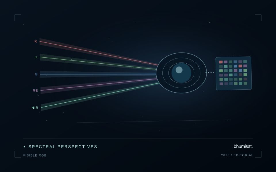
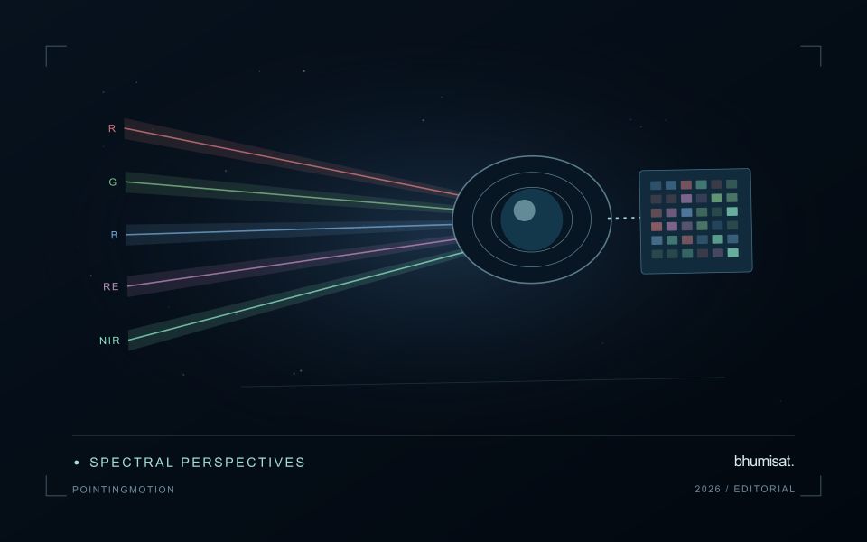
A surface does not necessarily reflect incoming light equally in every direction. Its measured brightness can change as the positions of the Sun, surface and sensor change, even when the surface itself is similar. The bidirectional reflectance distribution function provides a framework for describing this directional behaviour. In practical image analysis, the relevant lesson is that a difference between observations may contain a geometry effect as well as a real surface change. Canopy structure, shadows and surface roughness can all influence that relationship.
The magnitude and pattern of a geometry effect depend on the landscape and spectral measurement. A row crop, closed forest and exposed soil need not behave in the same way. Terrain introduces another layer because slope and aspect alter local illumination. A simple brightness adjustment is not automatically an adequate solution. A workflow should first identify the type of comparison it needs and whether the available product already includes a relevant normalisation. Applying an additional correction without understanding prior processing can create a new inconsistency.
Normalise geometry with a clear purpose
Geometry normalisation uses a model or adjustment to express observations under a more consistent reference condition. It is an approximation designed for a defined purpose, and its performance should be checked rather than assumed. Keep the input geometry, model assumptions and processing version where they are available. Compare representative surfaces before and after the adjustment. A useful test examines whether the correction reduces systematic variation in stable areas while preserving changes that are supported independently by management records or field observations.
For an agricultural service, the importance of this effect depends on the size of the change being interpreted. A subtle trend can be more sensitive to residual geometry variation than a major harvest event. Evaluate whether an apparent improvement in a time series survives across seasons and fields, including those with different canopy arrangements. Retain a clear explanation of what has been normalised and what remains uncertain. Viewing geometry becomes manageable when it is treated as part of the measurement context instead of being attributed silently to crop condition or land-cover change.
The setting: Cotton production fields
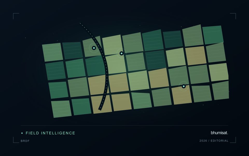
Cotton fields can differ in planting time, variety, stand density and management, producing different image trajectories through the season. A monitoring programme should organise those differences before deciding which fields are unusual. Early observations often combine crop and soil, while later management and crop-stage changes can alter the canopy in ways that require contextual interpretation. A reliable field calendar is therefore as important as the choice of a vegetation measure.
Compare observations that meet consistent quality requirements and inspect whether a mapped pattern persists across suitable dates. Field boundaries, tracks, wet areas and neighbouring crops can affect irregular management units. Record the valid area contributing to a summary, especially when clouds or shadows leave only part of a field visible. If several image products are combined, evaluate their alignment and measurement consistency before treating a difference as evidence of crop change.
A scouting visit should collect observations that address the intended decision, such as uneven development or a need for agronomic review. Record crop stage, recent operations and the sampling area consistently. An optical anomaly is not a direct measurement of fibre characteristics or a confirmed diagnosis of a particular problem. Models for commercial outcomes require corresponding reference data and independent evaluation, while inspection products can be assessed through their usefulness in directing representative and timely field visits.
Define a representative reference sample
A reference sample should represent the situations in which a method will be used. Begin by defining the target population: locations, time periods, management conditions, surface types, or instrument states that belong within the intended application. A collection of convenient observations may be valuable for exploration, but it does not automatically support conclusions about that wider population. Make the scope of the sample visible before calculating a summary of performance.
Consider a stratified design when important conditions are unevenly represented. Relevant strata might include different landscape types, developmental stages, observation quality levels, or ranges of the variable being estimated. Choose sample locations within those groups using a documented rule, and retain the information needed to understand their selection. Where access restrictions affect the sample, record the excluded conditions so that the limits of the resulting evaluation remain clear.
Keep development and evaluation evidence separate where the purpose of the study requires an independent test. Nearby observations or repeated measurements can share information, so a random split of individual records may overstate independence. A split organised by location, period, or operational unit can provide a more demanding comparison. The appropriate design follows the intended deployment, the structure of the observations, and the errors that matter to the user.
Maintain the geographic units of analysis
Many observation services summarise measurements within a field, management block, catchment, forest unit, or other mapped boundary. The meaning of that summary depends on whether the boundary accurately represents the unit being discussed. Start with a clear source for the geometry and record its date, coordinate reference, and intended use. A boundary drawn for visual orientation may require additional checking before it becomes a measurement unit.
Inspect overlaps, gaps, narrow fragments, and features that may have changed since mapping. A geometrically valid polygon can still describe an outdated operational unit. Ask the responsible team how divisions, mergers, new infrastructure, and management changes are recorded. Where pixels or reference measurements cross a boundary, define how they are assigned or excluded so that results remain comparable between analysts and processing runs.
Version the boundaries alongside the observations. If a unit changes, preserve a relationship between the previous and revised geometry rather than replacing the history without explanation. Comparisons through time should identify whether they use a constant spatial unit or the operational units valid at each date. This makes it easier to distinguish a change in the measured surface from a change introduced by the geography used to summarise it.
Bring the evidence back to the decision
A successful handoff leaves the recipient with a clear result, sufficient context, and a practical route for raising questions. Test the delivery with the people who will use it, including how they respond when observations are missing or qualified. Capture their feedback as evidence for improving the product. The most useful delivery format is the one that preserves the relevant technical meaning while fitting the decisions, time constraints, and responsibilities of its intended audience.
Sources & further reading
Explore the bhumisat spacecraft concept and our vision towards 2030, or return to the journal.