Remote observations show patterns, while practical decisions depend on explaining what those patterns could mean. Interpretation therefore requires more than locating a high or low value on a map. A useful analysis considers the timing of the observation, the physical processes that influence the measurement, and the information available from complementary sources. This perspective separates an observed signal from a proposed explanation and from an action recommended to a user. Keeping those stages distinct makes it easier to investigate alternative causes, communicate ambiguity, and choose a proportionate next step.
This working guide considers viewing geometry and brdf effects along changing sandy shorelines. The immediate decision is to review shoreline positions over time. Useful reference evidence includes acquisition context, field positions and consistent shoreline definitions. The case is an illustrative planning context, with assumptions to check against the actual sensor, landscape and project requirements.
The setting: Changing sandy shorelines
A shoreline is not always one fixed boundary that every observation measures in the same way. The visible water edge, a vegetation boundary and another mapped coastal indicator can represent different features. A monitoring programme should define its chosen shoreline consistently before comparing dates. Tidal conditions, wave state, seasonal beach changes and the geometry of the image can all influence the position recorded, even without a lasting change in the coast.
Spatial resolution and alignment determine the precision with which a boundary can be located. A sharply drawn line on a map should not imply more positional certainty than the observations support. Compare acquisitions under suitable conditions and retain the information needed to examine their differences. Mixed pixels, shadows and narrow coastal features may require manual review or an uncertainty zone rather than an automatic interpretation at every location.
Field validation should use the same shoreline definition as the image analysis and record when and how a position was measured. A visit under different water conditions may represent a different boundary even if its coordinates are accurate. Evaluate change over appropriate distances and periods, and avoid treating every small mapped displacement as erosion or deposition. A transparent product shows the observed positions, their dates and the uncertainty relevant to the decision being considered.
The observed surface has a direction-dependent response
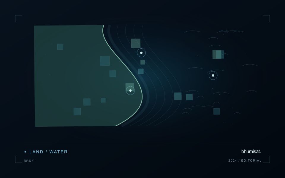
A surface does not necessarily reflect incoming light equally in every direction. Its measured brightness can change as the positions of the Sun, surface and sensor change, even when the surface itself is similar. The bidirectional reflectance distribution function provides a framework for describing this directional behaviour. In practical image analysis, the relevant lesson is that a difference between observations may contain a geometry effect as well as a real surface change. Canopy structure, shadows and surface roughness can all influence that relationship.
The magnitude and pattern of a geometry effect depend on the landscape and spectral measurement. A row crop, closed forest and exposed soil need not behave in the same way. Terrain introduces another layer because slope and aspect alter local illumination. A simple brightness adjustment is not automatically an adequate solution. A workflow should first identify the type of comparison it needs and whether the available product already includes a relevant normalisation. Applying an additional correction without understanding prior processing can create a new inconsistency.
Normalise geometry with a clear purpose
Geometry normalisation uses a model or adjustment to express observations under a more consistent reference condition. It is an approximation designed for a defined purpose, and its performance should be checked rather than assumed. Keep the input geometry, model assumptions and processing version where they are available. Compare representative surfaces before and after the adjustment. A useful test examines whether the correction reduces systematic variation in stable areas while preserving changes that are supported independently by management records or field observations.
For an agricultural service, the importance of this effect depends on the size of the change being interpreted. A subtle trend can be more sensitive to residual geometry variation than a major harvest event. Evaluate whether an apparent improvement in a time series survives across seasons and fields, including those with different canopy arrangements. Retain a clear explanation of what has been normalised and what remains uncertain. Viewing geometry becomes manageable when it is treated as part of the measurement context instead of being attributed silently to crop condition or land-cover change.
Budget the complete processing workflow
A processing budget should cover the complete path from source observations to a maintained product. Data access and computing are only part of that path. Include preparation, geographic updates, reference collection, expert review, delivery, and support where those activities belong to the service. A calculation that runs cheaply on a small demonstration can still require substantial effort when the surrounding work is repeated across many locations.
Measure representative tasks rather than assuming that every observation costs the same amount to process. Record data volume, processing time, retry frequency, manual interventions, and the conditions that create unusually demanding cases. Separate fixed setup work from work that grows with the number of observations or users. These records support decisions about batching, caching, storage policy, and the point at which a different processing design becomes worthwhile.
Connect the budget to a defined level of service. Faster delivery, more frequent observation, broader coverage, or more detailed review can each change the resources required. Describe these trade-offs before promising a delivery pattern that the workflow has not demonstrated. Review the budget using operational evidence and preserve enough detail to understand changes between processing versions. The aim is a sustainable service whose resource choices remain aligned with the information that users value.
Design an evaluation that reflects deployment
A model evaluation should resemble the conditions in which the model will be used. Start by identifying which relationships the development data share: nearby locations, repeated observations of the same unit, common collection teams, or measurements from a single period. These relationships can make records less independent than they appear. An evaluation that ignores them may test the ability to recognise familiar conditions rather than the ability to operate in a new setting.
Choose a split strategy that matches the intended transfer. Holding out locations, seasons, operational units, or acquisition conditions can answer different questions. Document which question each split is designed to address, and keep the held-out evidence separate while selecting features and tuning the method. Repeatedly inspecting the same evaluation set to improve a model gradually makes that set part of development, even if it retains its original label.
Report results at a scale that is meaningful to the user. A strong average can hide poor performance for important subgroups or unusual conditions. Examine error patterns and retain examples of both successful and unsuccessful predictions. Where the evidence covers only a limited range of conditions, describe that range explicitly. The evaluation then becomes a practical guide to suitable use, further testing, and the collection of additional reference observations.
Bring the evidence back to the decision
A strong interpretation states what was observed, which explanations remain plausible, and what additional evidence would help distinguish them. Avoid presenting a convenient label as a confirmed cause when the measurements support only a broader pattern. Connect the proposed next step to the significance of the decision and the confidence available. This creates an interpretation that a field team, analyst, or project partner can examine, challenge, and improve as further observations become available.
Sources & further reading
Explore the bhumisat spacecraft concept and our vision towards 2030, or return to the journal.